
Building Energy Modeling in OpenStudio
Building Energy Modeling in OpenStudio - Tutorial
Updated February 14th, 2025
In these YouTube videos we discuss the steps needed to create a building energy model using OpenStudio (and FloorSpaceJS, located within OpenStudio). We will be creating an energy model of a simple, rural fire station. The lessons progress from importing library files, creating geometry, setting site parameters, and creating schedules.
Building energy use is then calculated using the U.S. Department of Energy, EnergyPlus simulation engine via OpenStudio.
All software used for these calculations (SketchUp, OpenStudio, FloorSpaceJS, and EnergyPlus) are open-source and free to download.
1. Introduction to OpenStudio and EnergyPlus
4. Add Thermal Zones and Subsurfaces
14. Troubleshooting (Warnings and Severe Errors)
16. Add Domestic Hot Water System
17. Add Zone level Exhaust and Forced Air Furnace Systems
18. Add Zone level Basebaord and Unit Heaters and Packaged Terminal Air Conditioners
19. Add Dedicated Outdoor Air system
20. Review building performance by plotting EnergyPlus output variables using DView
21. Verify and adjust zone level air balance
22. Add transfer air to the model using EnergyPlus measures
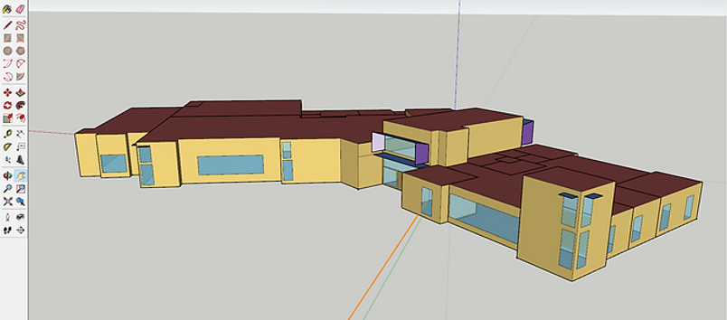
23. Modify the building geometry using SketchUp-1
Table of Contents:
1. Introduction to OpenStudio and EnergyPlusShort description about OpenStudio and EnergyPlus. This video will introduce you to a little of the history of energy modeling and describe some of the computational capabilities of the OpenStudio program.
So the question is: What is open studio?
Simply put, OpenStudio is a graphical user interface for EnergyPlus.
But, before we can fully answer this question, we need to know what energy modelling is and a little bit of its history.
I won't go very far back, just to the most recent and widespread use.
In the 1970s and 80s computer programs were created to simulate building energy use with the goal of reducing energy consumption.
By the 90s, the US Department of Energy had developed a robust program, free to the public, for this purpose.It was called DOE-2. Unfortunately, it required a lot of coding knowledge.
They further developed a graphical user interface called eQuest.Today, eQuest is the most widely used program for simulating building energy use.
It is free, however updates are no longer supported.
In the 90s, the Department of Energy began developing the next generation of energy simulation program called EnergyPlus.
Today it is the latest, stable building energy simulation program.
It allows engineers, scientists, and the construction industry to predict and simulate how a building uses energy through its lifetime.
Energy Plus uses a lot of complex mathematical models to calculate energy use for a building.
In addition, just like DOE-2, it is a very obscure, programming language oriented, program.
Not very user friendly.
By the late 2000s, DOE realized that in order to get widespread adoption of the program they needed to develop a robust easy-to-use graphical user interface.
They developed OpenStudio.
OpenStudio is a graphical user interface for creating inputs to EnergyPlus.
The workflow starts with creating geometry using Floor Space JS, located within the OpenStudio program.
Alternatively, if you have complex geometry you can use SketchUp and the OpenStudio plug-in.
Or you can import geometry from IDF files GBXML files, SDD files, or IFC files.
Then you can assign space types and thermal zones to your 3d model.
You could think of this 3D model as a shell that will later hold all of your energy modeling information.
From there, you can modify the model by changing different parameters such as:
How many people are in the building.
You can change lighting power densities. You can change ventilation rates.
You can change schedules for occupancy.
You can change other schedules, like when the building is open or closed.
You can change water usage or how many people are in the building at one time during the day.
You can change the HVAC systems set points. Basically, anything you can do in an energy modeling program.
You can do it in an OpenStudio. It is a graphical user interface so it is very intuitive.
Once you are done assembling the model of the building it exports it out to EnergyPlus.
EnergyPlus crunches the numbers for you and delivers information about your building.
The final result shows you lots of information like:Total and monthly energy use.
Building envelope performance.Peak space and HVAC loads.
Peak water usage and ventilation.
2. Building Energy Modeling in OpenStudio - Importing Library Files
In this video, we discuss how to import library files into OpenStudio.
Today, we are going to create an energy model for a fire station.
First we will start with opening a blank OpenStudio project.
Then we will save this as a new project in your project folder.
We will call it example 4. Save this? Yes.
We have a blank project here. There are no space types.
You can see when I click the space type tab, there are no space types.
First, we want to take a look at the project floor plan.
This will show us what types of spaces we have in this project.
There is an apparatus bay, decontamination laundry room, turnout locker room, corridor, storage, shower, office and a community room.
Next, we will import a library file that has the necessary templates.
Go to: File- load library and browse for the library file.
We will use a previous project for a fire station as the library file.
Click open. Now the library should be loaded.
To see the imported information, you can go to the library tab in the upper right.
We are on the space types tab, so we need to look in the space types library.
Scroll down to find the fire station space types.
Drag and drop the necessary space types into the project.
OpenStudio uses space types to encode information about how particular spaces are used.
This information includes loads such as people, lighting, infiltration, and plug loads as well as their associated schedules.
I will now add all of the space types we will need for this project.
You may skip ahead to 3:14.
Now we have all of our space types. The next task will be to add in a Construction Set for our fire station.
Select the Construction Sets tab on the left hand side.
Again, go to the library files at the right, select construction sets, and browse for our imported fire station Construction template.
You may skip ahead to 4:30.
Firestation, metal, right here. This is going to be a metal building so we will drop this Construction Set into our construction sets for this project.
Allow it some time to load.
Okay. Now we have a fire station, metal building. The exterior walls are metal, concrete slab, and exterior roof is metal.
You will want to double check that these constructions match those of your current project .
Next we will go to the schedules tab.
You will notice that many of the schedules have already been imported when we brought in the space types.
Occupancies, activities, lighting, etc.
Okay. That is how you load information from a library file.
Next episode will use FloorSpaceJS to create the building geometry.
3. Building Energy Modeling in OpenStudio - Create Geometry
In this video, we discuss how to create building geometry using FloorSpace JS within the OpenStudio application.
The next task is to create the geometry for the building.
First we will save the file as a new file. It is always good to save revisions of files in OpenStudio.
That way you can always go back to previous versions if you encounter trouble.
Next, we will check our Preferences-Units to ensure that we are working in the English Imperial system.
Next, we will go to the Geometry tab on the left.
Then go to the top where the Editor tab is. We will be using FLOORSPACEJS to create the geometry.
Click New. There are several options to create geometry and use references.
For now, we will just create a new floor plan.
Next select the Import Image button to import the floor plan.
You will want to move the floor plan to wherever your origin is.
We will use zero-zero as our origin. Try to locate it as close as possible.
Next, you will want to scale the image. You will notice that I put a scaling dimension on the image.
This allows us to have a reference for how large the space is.
Scale the image by dragging on the corner to adjust it to 120 feet.
Next, click outside of the image to lock it in place.
We will want to change our grid units to one half of a foot. To create a new space we will click the rectangle button.
Click and drag to create the space. When you want to add a new space, click the plus button.
You will notice that that the cursor turns red when it locks on to the edge of a previous space.
You may skip to 4:30.
The community room is an odd shape. We will create it by using multiple rectangles without clicking the plus to add space button.
You can see that the rectangles are additive.
Now we have our spaces.
Next, rename the spaces to reflect what is on our floor plan.
Click the expand button. Space 1-1 we will rename to 101 as seen on our floor plan.
Go through and rename all of the spaces.
You may skip to 6:00.
Next, assign space types to each space. Click the drop-down arrow to select the space that is applicable to that room.
For space 101, this is going to be the Apparatus Bay.
Do this for all of the spaces.
You may skip to 7:00.
Next, assign construction sets to each space.
Since all the spaces are contained within the same building we only have one construction set.
For this example we are not going to do a pitched roof or a blow floor plenum.
Check the floor to ceiling height.
Check the plenum heights. For the Apparatus Bay there is no plenum.
For the offices, lockers, storage, etc. we do have a plenum.
The community room does not have a plenum. We will not have floor offsets.
Now we are finished. Click Merge with Current OSM.
Now select the 3D View tab on the upper left. Our model has been created and space types have been assigned.
Next video we will continue with creating subsurface geometry on the model and other assignments.
4. Building Energy Modeling in OpenStudio - Add Thermal Zones and Subsurfaces
In this video, we discuss how to add thermal zones and subsurface constructions to the building geometry using FloorSpace JS within the OpenStudio application.
Now that we have created the building geometry, our next task is to add thermal zones and sub surfaces.
Again, we will create a backup file. Save as version 3.
Next, go to the geometry tab. Select the editor tab. It starts in the floor plan tab.
We have completed the floor plan and geometry. The next task is to assign thermal zones to each space or a collection of spaces.
Select the assignments tab. Expand the thermal zones tab and add a thermal zone.
We will call this thermal zone 101.
We need to know how many thermal zones there are.
Looking at the mechanical drawings, you'll note that pretty much every space has its own thermal zone.
Starting with the apparatus bay will do thermal zone 101.
We can click the duplicate button to create another zone. 102 and so on.
You may skip to 2:22
Now that we have created the thermal zones, we can contract the thermal zone tab by clicking this upper right button here.
We can assign the thermal zones.
For thermal zone 101 we select thermal zone 101 and then we select the space 101.
Select thermal zone 102. Select the space 102. And so on.
Now that we have added the thermal zones, we can move on to adding subsurface components.
Go to the components tab on the top. Select it. The first component that we will add is this door.
The door is approximately 7 foot by 3 foot.
Select the drop down menu. Select door. Click the plus button.
You can expand the menu here and you will note that this is approximately a 3 foot by 7 foot door.
To place the door, just hover over the top of the space.
You will note that there's an icon showing a door here with the approximate size.
Click to drop the door in place. Next, we have to add these windows.
These windows are approximately 3 foot by 6 foot.
Just click the drop down menu. Click window. Click + to add a window. 3 foot by 6 foot.
The sill height is approximately 9 foot high.
Again, go to the space, hover over the location, and click it to drop the window in place.
Do this for all the windows and doors.
For this door, it will be a glass door. We will duplicate one of the doors and change the type to glass door.
Same situation with this door.
Finally the overhead doors. We will select overhead door type.
That completes the addition of the windows and doors.
Click the collapse button to collapse the tab. You can now see that we have placed all of the windows and doors.
That concludes our lesson for today.
You will want to click the merge button again to merge the geometry with the open studio model.
Click the 3D View tab to see the final product.
5. Building Energy Modeling in OpenStudio - Site Tab
In this video, we discuss how to add a weather and design day file to your project. We also briefly mention some of the other information located on the site tab including measure tags, utility bill year vs. TMY year info, Daylight Saving, and Life Cycle Cost parameters, and utility bills.
Our next task is to fill out the information on the site tab.
We will save the file as a new version.
On the site tab you will see various information related to weather. The first task is to set the weather file.
We don't have any weather files for this project, so we will have to download them.
Go to the EnergyPlus website. Browse for the location.
We will say this project is located in Medford. We will use the TMY3 file.
TMY3 is the most up-to-date weather file data.
Click download all.
We need to take the data that we downloaded and drop it into the OpenStudio folder.
Browse to your local disk, go to OpenStudio, and put it into the EnergyPlus folder.
It is Energy Plus weather files, but we don't have a weather folder so we'll create one.
Next, go to Set Weather File. Browse to the location where we put this put the weather file.
Select it. The weather file is an EPW file. EnergyPlus weather file.
Next, import the design day file (.DDY).
It is one of the files that we downloaded. Browse to the OpenStudio EnergyPlus weather folder.
Select the ddy file. OK. The design day file is used for sizing the equipment that is specified as "auto size" in the project .
You can go through and look at the design day parameters.
You can even change some of these parameters to to suit your needs.
Another thing to note on the site tab is these measure tabs.
These will be used for advanced energy modeling. You can select the climate zones, but we will discuss these later.
The other task on the site tab is to select by year.
If you are going to model your your building based on specific utility data you would select this button.
But we are going to model our building using typical metrological year data. So, we will select this button here.
Our location in Medford is subject to daylight saving time. We will click this.
Double check that the beginning and ending of the daylight savings time is correct for your area.
The Lifecycle cost tab up at the top can be selected. This is for cost analysis on projects.
We will not cover that at this time.
Next tab is Utility Bills. You will note that you should select the specific weather year if you're going to input utility bills.
We will click this just to show you.
Click calendar year. We are going to model our building based on the year 2000.
Go back to utility bills. You will see that now you can input utility bills.
We will do this at a future lesson. Go back and select first day of year to model based on typical metrological year.
That concludes our lesson for today about the site tab. Please hit like and subscribe!
6. Building Energy Modeling in OpenStudio - Schedules Tab
In this video, we discuss the difference between schedule sets and schedules, how to alter and add schedules, and some of the different schedule types.
Next, we will look at the schedules tab on the left. Up at the top, schedule sets tab.
This tab shows schedule sets. You can think of a schedule set as a collection of various different schedules.
This schedule set will be applied to a space type.
A schedule set has various different schedules for people and loads located within a space.
For the fire station schedule set, we have: People occupancy levels throughout the day.
People activity levels in watts of heat output per person. We also have lighting watt density levels that vary throughout the day.
Electric equipment, gas equipment, water, steam, and also infiltration.
You can drop a schedule into a schedule set just as easily as going to the my model tab or the library tab.
Then dragging and dropping. We will do an example for this storage room schedule set.
If we had a gas equipment load located within the storage space we would just simply grab a gas schedule and drop it into the storage schedule set.
That is an example, but we don't have it for this project, so we'll delete this.
Creating a new schedule set is as easy as pushing the plus button and renaming it to whatever schedule you want.
Then drag and drop various schedules into the schedule set.
Next, we will go to the schedules tab. These are the individual schedules.
Look at this one. Always on. This is a common type of schedule used for energy modeling.
It is used to override equipment to ensure that the equipment is in the on position throughout the entire year.
The default schedule for this is 1.
We can create a new schedule just by copying using the x2 button.
We will call this Always Off. To change the value to 0, hover over the line and type in 0, Enter.
Now this schedule is always off.
There are different types of priorities located within within each of these schedules.
For example: If you have a specific override for sizing equipment using design day values you can create a custom schedule.
It is used just for sizing the equipment during a summer design and the winter design schedule.
Let's look at a different schedule. Clothing schedule.
Here, the default value is 1. Basically everybody in the building is wearing long pants, long shirts, and coats throughout the entire day.
You will notice that there's also a priority schedule. Click it.
This priority schedule is applicable between May and the end of September. The summer months.
This schedule is saying that during this period people located within the building are lightly dressed.
They are not wearing coats and they are probably not wearing long pants. They are wearing lighter clothing.
If we wanted to create a custom schedule, during the spring period, we would click the plus button.
Just copy Schedule Rule 1. Add it to the project.
This is called Schedule Rule 2.
We will do this for the spring months.
During the spring days, people will enter the building with coats and heavy sweaters on. It is cold in the morning.
Later in the day, they will remove some of the clothing.
To split the schedule, simply double-click on the line. We will change the morning hours to 1.This means that the occupants probably have long coats and sweaters on.
Around mid-day, the occupants shed those sweaters and coats as it gets warmer in the building.
That is an example of how to change the schedule.
Let us create a schedule for a thermostat set point.
You can simply go to the library we previously imported.
Let's look for a thermostat schedule.
For the Apparatus Bay, the temperature will be held constant throughout the year at a freeze protection set-point.
Just drag this this schedule from the schedules library and drop it here.
You will notice that it was dropped into our list of schedules. The default value is to maintain the space at 38 degrees.
Basically, above freezing. You will notice that there are two different priorities on the weekend.
Saturday and Sunday. On Sunday the space is held at 60 degrees.
This could be for some sort of gathering during Sundays.
Likewise, on Saturdays, the space is raised up to 70 degrees. Basically room temperature.
They must have some so sort of closed, indoor community gathering on Saturdays.
Let us create an HVAC setpoint schedule for heating. Click the plus button. Select the type of schedule.
Temperature. Click Apply. We will call this heating HVAC.
The building is occupied 24/7 and operational 24/7, so this will be a simple schedule.
All we have to do is hover over the line and type in 70 degrees. Enter. Room temperature.
That tells the HVAC equipment to maintain the space temperature throughout the entire 24 hours of the day at 70 degrees.
Let's create another schedule, but let's copy this schedule.
Push the x2 button. We will call this cooling HVAC.
Change this value to 75. We will say that cooling has a night setback just to save energy.
Double-click on the line to create a break.
Hover over the morning hours and type in 80. Enter.
Double click on the other side of the line to create a break. Hover over it. Type 80. Enter.
This sets the thermostat back during the night time. The building is being cooled to a higher temperature.
During the daytime the building is actively cooled and the cooling system essentially shuts off at nighttime.
If you want to look at the schedule in more detail you can zoom in using these buttons down here.
15 minute increments.
You can see it starts at 7 and ends at 5. You can also adjust by dragging the vertical line.
You can zoom in further to 1 minute increments.
Let's say the cooling gets set back at 4:28 in the afternoon.
That is how you create a schedule. Let us say there is a time during the summer where the fire station is closed for one week.
Let us create a custom priority override schedule. Click the plus button.
New profile? Yes. Click Add, then select the priority.
We will use a June shut down. The first week of June.
For the first week of June we don't need any cooling at all. We will say it is all week long.
Select all of these days. You will notice as you select those days, it changes over here.
This purple shows where the active schedule (that you're working on) is affected throughout the entire year.
We will override this to 80 degrees. There.
That is an example of schedules.
There are other different types of schedules. Laundry activity schedule.
This is basically saying how many watts of heat the people in the laundry room are producing.
Lighting schedules. This says the lights go off at nighttime.
They turn on at 8:00 in the morning. Then then they shut down at about 5:00 in the afternoon.
Gas schedules are similar.
Infiltration schedules are a fractional schedule. They are a multiplier that's affects the total space infiltration. When applicable.
There is also lighting schedules. You will see that the locker-room lighting goes on and off a lot in this schedule.
This is probably because the firemen are going out to various different calls throughout the day and night.
They have to use the locker room to get suited up.
So that is schedules in a nutshell.
Please remember to click like and subscribe if you like this video.
7. Building Energy Modeling in OpenStudio - Construction Materials In this video, we discuss the difference between material sets, assemblies, and materials, how to alter and add them, and how to access the Building Component Library.
Our next task is to review and edit the construction materials.We will go to the constructions tab on the left. You will see at the top there are several sub tabs.
Construction Sets, Constructions and Materials.Each of these is treated as a child-parent relationship.
Construction Sets are a group of construction assemblies that will be applied to the building.
You can see that, in this construction set, fire station metal, we have exterior surface constructions.
For the exterior walls we have metal building, concrete slab and metal building roof.
Interior surface constructions consist of an interior wall, interior floor, and interior ceilings.
Ground contact surfaces are all concrete.Exterior subsurface constructions consists of windows and doors and skylights.In addition, there are interior subsurface constructions. For example if you have interior partitions with windows or doors.
At the very bottom there are other constructions that may be applied.
A construction set defines a collection of constructions that make up the building.
They can be applied to the building or portions of the building. Next, let's look at the constructions tab.
The constructions tab shows construction assemblies. We will look at the first one.Metal building roof.
The metal building roof is comprised of metal roofing and roof insulation.You will see that these materials are applied in layers.
They will be used to calculate the thermal conductivity and heat transfer properties of this construction assembly.
The layer starts on the outside, metal roofing, and moves inward. Roof insulation, inside the building .
You will notice that there are measured tags. Recall we discussed these measured tags are located throughout the project.
These are for advanced energy modeling.Basically, you can apply measure tags to anything within OpenStudioAt the very end, you can use those measure tags as keywords that energy efficiency measures (EEM) can use.
The EEM can be applied to the project and automatically calculate how a building might be different if various variables are changed.
That is for advanced energy modeling. We will discuss that later. First, let's look at this metal roofing.
This metal roof is comprised of metal roofing and roof insulation 22.In order to find out what this roof installation 22 is, we need to go to the materials tab.
Select materials on the left, drop-down. Roof insulation 22.You can see that this roof insulation material also has measure tags. And it has thermal properties.Roughness. How thick it is. Thermal conductivity.
Density. Specific heat.Thermal, solar, and visible absorptance. You can see that the thermal conductivity and thickness combined together create an R-27 thermal resistance.Let us take a look at our project.
Our roof is composed of metal roofing, a thermal break spacer, and steel purlins plus insulation.Let us edit this roof assembly.
We will justWe are not going to be using this roof insulation for any other assembly, so just rename this: Purlins and Insulation R-29.
You will notice that the purlins plus insulation is approximately 10 inches thick.It has an r-value of 29.88 which is a 0.0028 thermal conductivity.
Let us change this 10 inches thick.0.0028 thermal conductivity. Now we have edited that construction material.Next, we also have to create that thermal break.
Duplicate this construction material. Select x2 and we will call this thermal break R-3.Looking at the thermal break, we have an R value of 3. It is basically 1/2 inch thickness and 0.1167 thermal conductivity.
Now that we've created those two materials, let's go back to the construction assembly for the metal roof.Select the constructions tab.
You will notice that we start with metal roofing, but then it goes directly to the purlins and insulation that we just edited.We need to put this thermal break in between.
First, let's delete this. Click the X. Next, go to my model, materials, and find our thermal break.
Drag it from our my model library and drop it into the construction assembly.You may have to click another assembly to refresh.
Click roof metal building again.You can see that it has been put in place. Select the purlins and insulation layer.
You can see that our metal building roof has been edited to include metal roofing, a thermal break, and purlins and insulation with an R-29 value.
That is how you edit materials and material assemblies.Rename this to simply Roof Metal Building.
If you go to the construction sets tab, you can see that it will automatically be updated because we just edited that construction assembly.
Roof Metal Building.If you do not want to go through the process of creating your own materials and assemblies:Look in the library files to search for a construction set that suits your needs.
The process is as simple as dragging and dropping in place.Go to constructions. Search for a roof.
We'll just use this as an example: R-31...R-25.We will just use this is an example.
Drag it and drop it into place.Now our construction set uses this roof instead of the roof we just created.
But we won't use this.Go back to my model, select constructions, drag roof metal building into place.
Similarly, you can do that for windows, doors, walls, and floors.If you do not have a material you are looking for, in your local libraries, you can search the building component library.
Go up to the top drop down, components and measures, and select find component.If you do not have the building component library access on your computer, you will need to register online.
Once you have registered online, the building component library will provide you with an authorization code.
Copy the authorization code, paste it into your BCL authorization key, and click OK.
This will give you access to the building component library onlineIt will take you to a new screen that allows you to search the building component library.
Suppose we wanted a window on the building component library that we don't have in our local library files.
Click the drop down on construction assemblies, fenestration, windows.You can search the online library for the specific windows that you are looking for.
Let us just select this one. Window, metal framing, all other, complies with 189.1 2009, residential, 2A climate zone.Click the check button and click download.When it is done downloading, you can close this window.
Next, go to your library tab, select constructions drop down, and search for the file that you downloaded.Right here.
We can use this and drop this into any one of the window categories.We will just use it for fixed windows for this project.
There.You can see that this is a building component library component because it's denoted with a BCL.
That is constructions, construction sets, and materials. Thank you. Please like and subscribe!
8. Building Energy Modeling in OpenStudio - Buildings Loads
In this video, we discuss the various thermal, electrical, gas, and water loads specified for the buidling. We will do an example of how to create a new load and how to import a load from a library file.
Next, we will look at the loads inside our building.
Select the loads tab on the left. These are all of the heat, electrical, gas, and steam loads located within the building.
There is also an internal mass definition for calculating thermal mass based on density of materials located within the building.
First, let's look at people definitions.
These are our occupant densities located within various spaces.
These loads calculate the number of people within a space and how much heat output each person provides to the space.
Also, carbon dioxide and what fraction of their heat they provide is radiant heat.
You can specify the occupancy by number of people, people per floor area, or floor area per person.
Let us look at light definitions.
Light definitions can be specified based on power, power per floor area, and power per person.
You can also specify what fraction is radiant,visible, and how much of that affects the return air to the HVAC system.
Let us do an example of adding an electrical equipment load.
Let us say we have a microwave located within the closed office.
Currently, the closed office does have an electrical equipment definition.
This is probably for printers, computers, and some other task lighting equipment.
We will use this as a template. Click the x2 to duplicate.
Rename this to Office Microwave.
The microwave is probably designated in watts. It's a 1200 watt microwave.
You can see when we changed it to watts, it actually deleted the watts per floor area value.
That is simply how you create a new space load.
However, the load itself has to have a schedule.
We will have to create microwave schedule located within schedules. Go back to the schedules tab.
Click + to add new object, schedule, fractional schedule.
Fractional indicates how much the microwave is being used throughout the day. Click apply.
Rename it to Office Microwave Schedule.
We will say the microwave is really only used for a few minutes at a time.
Probably during the morning hours. Only for several minutes.
You may skip forward to 6:00.
Used during lunch time and in the evening.
Just use the default schedule for simplification.
That is how you create an office microwave schedule.
Later, we will apply this schedule and the load to our space type.
Let us go back to the loads tab. There are also other loads that will be applied later in the project.
That is how you create a space load.
You may also drag and drop loads from your loaded library files.
Go to the library tab. We'll do an example of a light definition.
Scroll down to light definitions. Browse for the lighting load definition that you would like.
We will just use this here. Mid-rise apartments, corridor lights. Drag and drop the definition from the library.
You will note that it has been added to our project.
Again, you will have to create a schedule for this, because later we would assign this load to our space.
But for now, we won't be using this.
We can use the Purge All Unused Objects button down here to purge all unused definitions that are not being applied for this project.
Or you can select this particular load and just click the
X button to delete it. We will purge unused objects.
Using the Purge All Unused Objects button helps us reduce some of the clutter in our project.
It is good practice to go through some times and just double check that you haven't got a lot of unused items. *Oops! Be careful not to purge items that have not been assigned to spaces!*
That is the loads tab. Thank you. Please like and subscribe!
9. Building Energy Modeling in OpenStudio - Space Types
In a previous video, we imported space types for our project. In this video, we will revisit the space types tab and discuss how building constructions, loads, schedules, and infiltration are assigned to a space type.
Next, we will revisit the space types tab.
Select the space types tab on the left.
This is where we originally assigned space types to this project.
If you would like to recall how to install space types, please review the previous video.
Looking at these space types, you will notice that there is a default construction set, but it is empty.
We need to assign a construction set to all of these spaces.
Go to the my model tab.
Drop down construction sets.
Drag and drop our single construction set.
To apply that construction set to all of the other space types. Click the check boxes.
Select the construction set you want to copy. Click Apply To Selected.
It automatically populates the construction set to all of the space types that were selected.
This construction set is basically saying what type of constructions these spaces will have.
You can customize these by creating additional construction sets.
To create additional construction sets, please see the previous video.
Next, you will notice that the space type has a schedule set and an outdoor design specification outdoor air.
This is the ventilation specification. It tells the energy model how much ventilation is required for that space.
On this column, you will see space infiltration design flow rates.
The space infiltration design flow rates are also specified.
You can change the flow rates based on floor area, total space, exterior surface area of roof and walls, exterior walls, or air changes per hour.
To create a different infiltration rate, just rename it and change the values to what you want.
Similarly, you can copy those just like we just did with the check boxes.
We will apply an infiltration rate to the space plenums.
You can see the final column is a Space Infiltration Effective Leakage area.
We will not be using this, but I will illustrate how to find information about this input for the program.
Search for Space Infiltration Effective Leakage Area in your browser.
You are going to want to look for Big Ladder Software or EnergyPlus input/output.
We will look at Big Ladder Software because they have the EnergyPlus input/output located online (HTML).
Next, select Effective Leakage Area or you can click the link.
This describes what the Effective Leakage Area is.
Essentially, it is saying that this is a different way to calculate infiltration rates and it is normally used for smaller residential type buildings.
We will not be using this for our project.
We will only be using Space Infiltration Design Flow rates.
Next, you can go to the loads tab up at the top to see what type of loads have been applied to the each individual space.
For our Apparatus Bay, we have lighting load definition and an associated schedule for lights.
Likewise we have electrical equipment loads. This is the definition and this is the schedule.
We also have the same for infiltration. A load name and the schedule.
You will recall in a previous exercise we created a microwave load.
That was to be applied to the closed office.
You will note that there is no microwave load on the office so we will have to drag that into this space type definition.
Go to the my model tab. Browse to electrical equipment definitions.
Locate the microwave in the Electric Load
Definitions.
It appears that we may have deleted our microwave load definition. Or, we purged it in the previous exercise.
Let us add that back into our loads.
Select the loads tab, electrical equipment definitions, copy this, rename it.
Next, go back to the space types tab.
Select loads, scroll down to closed office, go to my model, electric equipment definitions.
Drag and drop the microwave into the closed office space type.
You will note that the microwave has been automatically assigned the fire station equipment schedule.
We need to change this to the microwave schedule that we created.
Go to my model and browse down to the rule set schedules.
Look for the microwave schedule that we created.
Drag and drop that next to the microwave load that we installed.
Now the microwave load and schedule has been applied to that space type.
You can see this has a multiplier.
This is used for fine-tuning a model without having to change loads or schedules.
If we discover that the microwave is actually being used half as much as what what we thought, we can change this value.
The energy model will automatically apply a 1/2 multiplier to it.
We will not do that here.
You will note that the default values are green and any overridden values have been changed to black.
That is how you add loads and loads schedules to a space type.
There is a filter button up here. For very large projects that comes in handy.
For example if we wanted to just look at occupancy loads we can filter by people.
For lighting loads, we can filter by lights.
Up at the top, the Measures Tag tab also is comes in handy for advanced energy modeling.
As discussed, these are keywords that energy efficiency measure (EEM) programs use to change the energy model.
They are use it to see how it affects energy use of the building.
The Custom Tab, I believe, is used for custom programming.
I will briefly discuss how to create a new space type.
Click the + button. Rename the space type to what you would like. We will call this Workshop.
Next, apply a construction set. Apply a schedule set. Apply a specific outdoor air.
We will just copy or we can select a different one.
Let's go to the library tab, specification outdoor air.
We will just do mechanical room ventilation.
Look for an infiltration design flow rate.
Look for mechanical room...
How about Utility.
Next, go to the loads tab.
Locate your new space type, Workshop. Drag and drop loads into the space.
This will be a Machinery room so we won't have a people definition.
We will do lights definition, storage and electrical equipment utility.
Finally, we want to assign an electrical equipment schedule.
To do that, go to my model, rule set schedules.
We will just say that the electrical equipment is always on.
That is how you create a space type.
To delete it, simply push the X button at the bottom.
Sorry.
Click the checkbox and then push the X button.
Thank you. Please like and subscribe!
10. Building Energy Modeling in OpenStudio - Geometry Tab
In a previous video, we created our building geometry. In this video, we will revisit the geometry tab and discuss additional features for viewing and editing the 3D model with FloorspaceJS.
Next, we will go to the geometry tab. At the first tab is 3D view, in geometry.
This allows you to inspect the building model. Using the right mouse button you can pan the model across the screen
Using the middle mouse button you can zoom in and out. Using the left mouse button you can rotate the model.
Over here are some additional controls. Changing the orthographic control changes the perspective of the model.
This can be useful for selecting specific items based on a view.
Let us do the X view. You can see that without orthographic turned on, it shows a more perspective view.
Next, there's some additional functions that act as filters or rendering. Right now we have it rendered as a surface type.
You can see that the roof is colored a beige color. The walls are brown. Glazing and glazed glass doors are a more transparent color.
The overhead doors are a dark brown color. The ground floor is a gray color.
If we change the render mode to “normal”, this is for rendering based on how the surfaces are oriented.
Right now all of our surfaces are oriented properly.
Let's get rid of walls. You can see that all of the outside surfaces are gray and all of the inside surfaces are red.
If one of our surfaces was accidentally flipped, we would see it show up as red on the outside.
That tells us that we need to correct its orientation in the geometry editor.
Next, if we go to boundary rendering, this shows you how the energy model will be rendering.
How the energy model will treat the surface. Most of the blue is an exterior surface.
Let us get rid of walls. Again, you can see that the interior surfaces are green.
Let us get rid of roof. The interior walls are green. The interior floor is brown. I'm sorry the the ground floor is brown.
All of the exterior wind exposed and sun exposed surfaces are blue.
Next, we'll look at render by construction. This tells you what type of construction it is.
The purple are windows. The teal color is an opaque door.
We also have glazed glass doors which are colored white. The exterior walls are a grayish Brown.
The roof is colored pink and the ground floor is colored Olive.
This will help you tell if you have additional construction materials located throughout the building that have been specifically assigned to specific spaces.
Next, let's look at render by thermal zone. This shows you all of the thermal zones located in the building.
These these are the thermal zones that we assigned in the very first lesson.
You can also see if there are different spaces, but there they might be combined into a single thermal zone.
Next, we will look at space types. This renders by space type. you can see the Apparatus Bay is green.
All of our plenums are a dark red color. We also have storage space, office space, locker, restroom spaces, and a community space.
We can also render by a building story. However, for this example we only have one building story so it only shows one color, green.
As discussed, you can also apply filters such that you can't see certain surfaces or sub-surfaces.
If we wanted to get rid of the roof we would uncheck the roof so we can see inside the building.
Let us switch back to render by surface type. Likewise, you can remove the doors and windows.
If you do have shading objects in this file, you can hide them.
But we don't have that in this model. That will be a for a future lesson.
If you have partitions located inside the model, for example office cubicles, those would show up here and you can hide those.
We don't have those in this model. Finally, you can click this button to show as a wire wireframe.
Although I don't know how to use this.
Next, let's go to the editor tab. We will discuss some of the additional functions of FloorspaceJS.
Let us do an example for this space here. It is actually comprised of two separate spaces but we originally just created one large storage space.
Let us split this into two. First, we will want to delete this space 105/106 as well as the plenum 105/106.
Next, we want to draw in a new space. Click the plus button. We will use the polygon tool this time.
Click to begin the polygon, click, click, click, and to complete the polygon click at the very first spot.
Next, create the tools 106 room. Whoops. Messed up. Let us use the undo button.
Create one more space. Next, we will have to rename these and add in the plenums. Space 1-1...
Okay, it appears that the program is moving slowly, or it's even frozen.
We can wait for it or we can try a different approach. Let us go ahead and reopen this.
Go back to the geometry tab. You can see that none of the changes were changed on this.
Click Save and go to the file folder of the project that you're working on.
Go to the open studio folder where all of the project files are located. Find the floorplan JSON file.
Open it in a text editor. Change this show import/export to read TRUE.
Save it. Then we will open this floorspace JS file using an online version of floorspace JS.
To do that, open a web browser. Browse to unmethours.com.
This will be a good exercise to show you how to troubleshoot problems.
Unmethours.com has a lot of people that use OpenStudio and EnergyPlus for energy modeling.
If you have questions, it has probably already been answered on unmethours.
We will just search for “FloorspaceJS freezing”. Select this topic. You can read through it.
Basically, FloorspaceJS development team has created an online version of Floorspace JS.
It uses Javascript, so any web browser can open it.
We will open this link to FloorspaceJS and we will open our file.
Browse to the project folder where the file is located. Click open. Now we can see our floor plan.
Delete this plenum. I'll show you additional functions that FloorspaceJS has.
We are editing these two storage rooms, so let's use the eraser this time.
I'll show you how the eraser works. Simple as that. It erases the space.
Then, we will go back to the polygon tool...well...sorry let's duplicate this storage room.
Then we will go to the polygon tool to create a new storage room. The duplicate tool is very powerful.
It allows you to duplicate all of these items that were filled in before, so that you do not have to refill those in.
We have now split this room into two. Next, go to assignments.
Let us see. We will have to create a new thermal zone for this new space.
There. Let us go back to floor plan now. I'll show you some additional functionality that FloorspaceJS has.
If you wanted to create another story for the building, simply use the duplicate tool.
It places the next story right above the first story. You can edit the attributes of the stories using the expand button.
An additional function that FloorspaceJS has: this fill tool.
If you have a story above another story, you can use the fill tool to simply copy the previous space below up to the space above.
This Apparatus Bay, on Story 1. If we just click the fill tool, and click, it creates another Apparatus Bay above, in Story 2.
We can expand this and look at the space. Oh. Excuse me. It just creates a space.
You will have to go through and fill in space type, construction set, thermal zones.
For this project, we won't be using a second story, so we will just go ahead and delete story.
Ok. Once you're done editing the floor plan, we can go up to the top and click Save Floorplan.
Click download. This will download into your downloads folder.
Next, go back to the project folder where your OpenStudio files (and .json file) are located.
Go to your downloads folder. Cut and paste this .json file into your OpenStudio folder.
We will want to replace the file.
Next, go back to OpenStudio and reload the project. Go back to geometry tab. Go back to editor.
Okay. You can see that these are the spaces that we created using the web browser version of FloorspaceJS.
We will just do a preview. This is good to hit. This button...it...
I am not sure what it does, but it refreshes the 3D model. You can see that those spaces have been added.
We will click close. Merge with current OSM. Click OK.
Now we can go back to the 3D view and we can see that those spaces have been edited.
The last task: go to spaces tab. We will rename those spaces that we created. this one was 105.
This one was 106. This is 106 plenum. This is 105 plenum. Go to thermal zones tab.
You will see that FloorspaceJS created a bunch of extra thermal zones. I'm not sure why.
It is a glitch.
You can simply get rid of those by doing purge unused objects.
Finally, we will save the OpenStudio file. Go back to geometry tab. Review our geometry.
You can see that the floor plan has been edited.
Thank you. Please like and subscribe!
11. Building Energy Modeling in OpenStudio - Facility Tab
In this video, we will discuss how to orient our building relative to North. We will set defaults for space, constructions, and schedules. We will add exterior lighting. We will also briefly discuss adding stories to the building and adding shading elements.
The next tab is the facilities tab. Go to the left and select the facilities tab.
On this tab you can change the building name. We will call this Rural Fire Station.
Next, you can see there are measures tags, just like we discussed previously.
Energy Efficiency Measures (EEM) can use these as keywords to change parameters of the model.
That is for advanced energy modeling. Next, you can see the north axis as set at 0.
Going back to the geometry tab, we can see that the north axis is currently set on this green axis line.
If we wanted to orient the buildings such that the north axis was on the red axis line, we would have to adjust this by 90 degrees.
Going back to the facility tab, you can change this to 90 degrees.
Next, you will see that there are three different defaults that you can add from your libraries.
This is the power of OpenStudio. OpenStudio fills in information from a top-down approach. Parent-child relationship.
This is the very top. At the very top, you can fill in space types, construction sets, and schedule sets.
I went through and deleted some of the information in our file to illustrate this example.
Let us go to spaces. You can see in the spaces tab that I have removed some of the information.
Space type for the Apparatus Bay is not there. The default construction set and the default schedule set is not there.
If we go back to the facility tab and add those into the top, all of that information will be defaulted to these default values.
Go to my model tab, space types. We will say the default space type is an Apparatus Bay.
Construction Sets. We only have one. Metal fire station. Schedule sets. We will just use the default fire station schedule set.
Go back to spaces.
You will note that the space type for the Apparatus Bay has been populated but the default construction set and schedule set have not been populated.
That is because all of these are empty and they will use the defaults for the facility.
The ones that we just dropped into this space right here. These spaces.
Let us go to the stories tab.
You can add additional stories to your building if you haven't already done those using FloorspaceJS or some other different geometry editor.
Let us go to the shading tab. The shading tab is used for adding additional geometry to your model that is not actually within the building.
It does not affect and does not create exterior loads such as lights or exterior equipment.
You could think of shading as adjacent buildings and trees that shade the building throughout the day.
Shading would reduce cooling loads.
We will not be using shading in this model. We will do that in an advanced lesson.
Let us go to exterior equipment. Here is where you can add exterior lighting to your building.
Let us say we have a couple of small lights on the exterior for security.
Click the + button to create new exterior lights. It automatically populates it with a load definition.
Click the load definition and we will say that total wattage is 400 watts for exterior lights.
Next, go to schedule. The default schedule is set for always-on. Discreet.
If you wanted to edit this schedule, you can go to the schedules tab and modify it.
Next, we will look at the control option. Control option specifies that the lights go on based on the schedule only.
Alternatively, you can select astronomical clock. Using this combines the two.
So you will have a lighting schedule for the lights going on and off and the astronomical clock will override that schedule if it senses daylight.
Thus, turning the lights off during daylight hours.
The astronomical clock is a photocell that shuts the lights off during daylight hours.
Next, you can do a multiplier just like we have multipliers elsewhere. This will multiply the wattage.
And, there is an end-use subcategory. The end-use subcategory is used for sub-metering.
If we wanted to have an additional electrical meter to track the energy use for the lights, we can rename this to general ext lights.
That is the facility tab. Please like and subscribe! Thank you.
12. Building Energy Modeling in OpenStudio - Spaces Tab
In this video, we will discuss the parent-child-inheritance relationship of OpenStudio entities. We will also show how to edit spaces, loads, surfaces, and sub-surfaces at the lowest (space) level of the energy model.
Next we will discuss the spaces tab. Up at the top we will start at the properties tab.
This is a list of all of the spaces that you have in the project.
As discussed in the previous video, these empty spaces will be filled in by information collected from the next level up.
The spaces tab is basically the lowest level there is.
So, if there is a particular space that has a particular load or construction type, and it's not the same as all of the rest of the spaces, then you would insert it here.
If you go to the air flow button, you can see infiltration and outdoor air object
names.
These were edited in the previous video when we discussed space types on this space type tab.
Again, all of this information will be populated from a higher level of information source.
Let us go to the loads tab. This shows all of the information that has been collected from higher level information sources.
If we had two different spaces there were exactly the same space type; for example our storage rooms 105 and 106.
But, if only one storage room had a microwave we could simply drag and drop the microwave into that space.
Go to the my model tab equipment definitions, microwave, and you can drag and drop it to the space 105.
Likewise, you would have to do the schedule for the microwave as well.
So, that differentiates this storage space from this storage space.
But let us delete this example.
Next, we can go to the surfaces tab at the top. The energy model is comprised of surfaces and sub surfaces.
Surfaces are the main surfaces of the building walls, roofs, floors, and ceilings.
Let us look at this. This is the Apparatus Bay. Let us say this apparatus Bay had a different roof than all of the rest of the building.
If we go to the library tab and look for constructions we can apply a different roof type to this apparatus bay.
You can see that it is now changed and it is not green anymore. It is black.
We have overridden this default value. If you want to return it to the default value, select the item and then push the X button up on the top right.
You can see that it's now returned to the default value. you can do this for all of the surfaces.
You can also do it for sub surfaces. Go to the sub surfaces tab at the top. Sub surfaces are all of the windows, doors, and skylights.
Also, interior windows and doors. On the building, sub surfaces are treated as children of surfaces.
Here, we can double check the constructions of all of our sub surfaces. For the overhead doors, the construction type is empty.
This means that we have not defined a construction assembly for overhead doors.
Let us go back to the constructions tab and take a look. If you look at exterior or subsurface constructions, overhead doors is missing.
We can choose to apply these overhead doors constructions from the construction set, which governs the entire project.
Or, we can apply that construction assembly just to the apparatus Bay by going back
to the spaces tab and editing these sub surfaces.
Go to library, constructions, and browse for a door type or alternatively you could create your own. Drag-and-drop in place.
Applying constructions that this sub surfaces level on the spaces tab applies it to a single, individual component of the entire building.
So, for these overhead doors, we will apply these at this level.
To copy to the other overhead doors, simply click the checkboxes, highlight the item, apply to selected.
Let us look at the other assemblies. Glass doors. It looks like glass doors are also not
defined.
Let us got back to our constructions tab. Glass doors. These are also not defined.
To define the glass doors for the entire project, go to my model tab and browse. We will just browse for a typical window.
Let us just use this one. This will apply to all the glass doors in the entire project as long as this construction set is set as the default construction set on the facility tab.
Going to the spaces tab again we will look at sub surfaces and scroll down. You can see that those boxes have been filled up with the default glass doors.
Some of the other buttons up here are for additional energy modeling. We will cover those in a later lesson.
Selecting interior partitions tab at the top allows you to edit interior partitions. We don't have these in this model.
Interior partitions are usually modeled as partial height walls. For example, like an office cubicle. We don't have these in this project.
The shading tab is also at the top. We don't have shading, but if we had individual shading objects we could edit those on this tab.
That is all for the spaces tab. Thank you. Please like and subscribe!
13. Building Energy Modeling in OpenStudio - Thermal Zones Tab
In this video, we will discuss how to rename thermal zones and add thermostat schedules. We will also discuss equipment sizing parameters and the use of ideal air loads.
Adding HVAC systems to the energy model will increase its complexity. We have turned on ideal air loads.
So we will just run the energy model and resolve simple errors before we start adding more complexity to our model.
Let us go to simulation settings and time steps. This sets the number of iterations that the program runs the energy model per hour.
The number of iterations per hour is set for six time steps per hour.
So, it simulates the building every 10 minutes. Let us reduce this down to one time step per hour.
This will speed up our calculations. We can always come back and adjust this later.
Next, let's go to measures. We want to add Diagnostics to the measures tab.
Go to the right and select drop down, reporting, drop down, QA/QC.
Select this Add Output Diagnostics.
If you do not have it, go to the bottom and click the Find Measures On BCL button. Browse to reporting, QA/QC.
Search for "add". You can find it right here. Add Output Diagnostics.
You can see it is checked because I have already downloaded it. If you do not have it, it will not be checked.
Check the check box and click the download button.
When you're done downloading, drag and drop the Add Output Diagnostics to the EnergyPlus measures.
This adds additional diagnostics when running the energy model to help troubleshoot problem areas.
Next, we will go to run simulation. Click Save and hit the Run button.
You can see that the simulation has failed. There are various errors associated with a failed simulation.
This will be good a good exercise. First, browse to the folder where your energy model is located and open the program folder.
Browse to "run" folder and select the EPLUSOUT.ERR file. Open it with a text editor.
There are two different types of errors. There are warning errors and there are severe errors.
Severe errors will terminate the program before it has finished modeling the building.
Most of these are warning errors. First of all, let's address the severe errors.
Scroll down until you find a severe error. You will note here is the severe error.
This says we were having a convergence problem with one of our building materials. Roof Metal Building.
This is one of the assemblies that we created earlier in the process. If you remember.
Let us go ahead and take a look at this and troubleshoot.
Go back to your materials tab on the left. Go to materials tab, drop down materials.
We will browse for thermal break, purlins and insulation.
These are the two materials that we created. Look at the thermal break.
We will take a look at what our calculations were for the insulation value.
The thermal break is 0.1667 and 1/2 inch thick.
And purlins and insulation...Should be 0.335. That should fix the severe errors.
Double-check that you don't have any other additional severe errors. We only have one.
Close the error file. Save the project. Rerun the simulation.
Success! We did have a proper simulation. However, there were several errors in in the error file that we noted prior.
Let us go back and look at the error file again. There are warnings.
The first warning: requested number of time steps is less than the suggested minimum of four.
This is saying that the program recommends using at least four time per hour.
We will ignore this one. Next let's look at the next warning.
This has to do with our cooling HVAC default schedule. It looks like these are similar.
The fire station locker occupant schedule. It looks like these schedules are not falling within our time step.
If we go back to the locker schedule, as an example, you can see these time steps are in very small increments.
Small enough that they start and stop within the hour.
But if you recall, our simulation settings were set to simulate every 60 minutes.
So, our simulation timesteps are not small enough to capture the on-off nature of the schedule.
That is what this error is saying. We can ignore this for now.
The same thing goes for the microwave schedule.
The next warning is always on, always off, and always on continuous.
These are integral schedules to the OpenStudio program. We can not edit these.
We will ignore these warnings.
The next warning is saying that there were no ground surface temperature schedules associated with our energy model file.
Therefore, the program will be using the default constant temperature throughout the year, which is 18 degrees Celsius.
That is not concerning. Let us go on to the next warnings.
These are check coincient / collinear vertices warnings. Collinear points.
This is saying that some of the vertices in our 3D model have been doubled up.
EnergyPlus does not like to have vertices doubled up. On top of each other.
For simplification, EnergyPlus deletes some of these vertices.
We don't have to worry about that warning.
Let us look at the next warning. It says there are 9 nominally unused constructions in input.
Some of these constructions are not being used inside our model.
Interior windows, partitions, and doors. We don't have any of those in our model.
Let us go back to the Construction Set tab. We do have exterior walls, floors, and roofs.
We do have interior walls, interior floors, and interior ceilings.
Ground contact surfaces, We do not have any walls in contact with the ground.
We can delete this. We do have interior floors that are in contact with the ground.
We do not have ceilings in contact with the ground. We do not have operable windows.
We do not have tubular daylight domes. We do not have tubular daylight diffusers.
We do not have any interior windows or doors. We do not have any interior partitions in our project.
We can delete that as well.
Next, go to the constructions tab and we can simply go through and Purge Unused Objects.
Select each one of the categories and click the Purge Unused Objects button.
Next, go to the materials tab and do the same thing.
This helps get rid of some of the clutter in our project and speeds up the simulation.
Save the model. Let us continue on with our errors and warnings.
This warning says that we're having comfort related issues but there is no comfort model selected.
This is for small hotel laundry. We are also getting the same issue with the locker room.
To fix this issue let us go to the space types tab.
Go to loads. This has to do with occupancy schedules.
In the laundry room. The decontamination room.
We have a laundry occupancy schedule that shows Work Efficiency, Clothing Insulation, and Air Velocity schedules nameed.
If we select our load definition, you will see that we do not have any comfort analysis selected for this.
Click the plus button and drop down thermal comfort model type.
We will just select the first instance.
This has to do with the laundry and the locker room. Locker room...outpatient...fire station locker room.
Plus. Add/Remove Extensible Groups. Select a Thermal Comfort Model Type.
That should solve those two warnings.
Let us continue with the additional warnings.
This warning is saying that the office corridor zone does not have any exterior walls so it cannot calculate an infiltration value.
You would have to do a different infiltration value for that type of space located on the interior of the building.
Let us look at it. Corridor. People infiltration.
It is selected as a flow / exterior area value.
You can change the infiltration value to flow per space, flow per area, or air changes per hour to ensure that that space receives some form of infiltration.
We can just ignore that error.
Same thing goes for the other interior rooms. Locker room, the restrooms, and the storage room.
Let us look at the next warning. Calculated design cooling mode for thermal zone is 0.
Thermal zone 101. Let us go to our thermal zones tab.
Thermal zone 101 does not have a cooling thermostat schedule, but it is trying to calculate cooling.
This warning is saying: with no thermostat schedule, the cooling load would be 0.
Let us continue on.
Same issue. Ideal air loads is trying to calculate a cooling load, but there is no thermostat associated with that space.
Let us look at the next issue.
This is saying that there are multiple electric meters specified, so it will report both meters.
Let us go to the next warning. These warnings have to do with life cycle cost analysis.
It does not have any energy costs to input into the model. We can ignore those warnings.
Next, let's go to these other errors.
This says there are ten unused schedules in the input.
To see what those schedules are, we would have to select "display unused schedules" in Output Diagnostics.
Let us do that. Go back to the model.
Click Save. Go to measures. Select Add Output Diagnostics. Click the drop down.
Select Display Unused Schedules. Save. Let us run the model again.
Go back to the error file. Open it. Scroll down to where we left off.
The following schedule names are unused schedules.
We are not using always off, laundry equipment gas schedule.
We can go back to our energy model. Go to the schedules tab. Select schedule sets tab.
Go to the storage room. You will note that the storage room has an occupancy schedule associated with it.
Look at our space types tab. Go to the storage room.
You will note that there is no occupancy assigned to that room.
The same situation goes with the apparatus Bay.
Going back to the schedules tab, we can get rid of those.
Go to the storage. Remove the occupancy schedule.
We will not need activity schedule. And, there is no electrical equipment in the storage rooms.
We can remove that as well. Go back to the apparatus Bay schedule set.
We do not need the occupancy or the activity schedules.
Next, go to the schedules tab.
We can go through and purge all of the unused schedules using the purge unused objects button.
Click save. Rerun the model.
Let us go back to the error file and scroll down.
This is still saying that there are some unused schedules.
Again, these are the schedules that are integral to OpenStudio so we can ignore those.
They are not being used anyway.
Next, look at this warning. These are unused schedules. They are not being used.
This is the clothing schedule that we created in the first lessons. Let us go back and look at that schedule.
Go to the schedule tab, clothing schedule. Let us troubleshoot this.
We have not applied this schedule to any days of the week.
We do have it applied through a date range, but we do not have it applied to any of the days.
We can select all of these days to make this applicable.
Let us look at schedule Rule 1. Do the same thing. Save.
That should solve all of our errors. Let us rerun the model and see if that fixed our problem.
This is a good exercise. With energy modeling, there is always troubleshooting to be done.
Go back to the error file. Open it up. Scroll down.
It looks like that solved our problem with the clothing schedule.
These final warnings are saying that there is a surface, but it does not completely surround the sub-surfaces.
This has to do with our doors. The doors touch the very bottom edge of the surface.
They are only surrounded by three sides. We can ignore these warnings.
This gives you a summary of all the errors and warnings.
The key problems are the severe errors that will stop your program.
Some of these warnings are not very problematic.
Some of them will help you ensure that your model turns out the way you intended it to be.
Let us close the error file. We can go to the results summary to finally see our results for the model.
We will go through this in the next lesson.
Thank you. Please like and subscribe!Adding HVAC systems to the energy model will increase its complexity. We have turned on ideal air loads.
So we will just run the energy model and resolve simple errors before we start adding more complexity to our model.
Let us go to simulation settings and time steps. This sets the number of iterations that the program runs the energy model per hour.
The number of iterations per hour is set for six time steps per hour.
So, it simulates the building every 10 minutes. Let us reduce this down to one time step per hour.
This will speed up our calculations. We can always come back and adjust this later.
Next, let's go to measures. We want to add Diagnostics to the measures tab.
Go to the right and select drop down, reporting, drop down, QA/QC.
Select this Add Output Diagnostics.
If you do not have it, go to the bottom and click the Find Measures On BCL button. Browse to reporting, QA/QC.
Search for "add". You can find it right here. Add Output Diagnostics.
You can see it is checked because I have already downloaded it. If you do not have it, it will not be checked.
Check the check box and click the download button.
When you're done downloading, drag and drop the Add Output Diagnostics to the EnergyPlus measures.
This adds additional diagnostics when running the energy model to help troubleshoot problem areas.
Next, we will go to run simulation. Click Save and hit the Run button.
You can see that the simulation has failed. There are various errors associated with a failed simulation.
This will be good a good exercise. First, browse to the folder where your energy model is located and open the program folder.
Browse to "run" folder and select the EPLUSOUT.ERR file. Open it with a text editor.
There are two different types of errors. There are warning errors and there are severe errors.
Severe errors will terminate the program before it has finished modeling the building.
Most of these are warning errors. First of all, let's address the severe errors.
Scroll down until you find a severe error. You will note here is the severe error.
This says we were having a convergence problem with one of our building materials. Roof Metal Building.
This is one of the assemblies that we created earlier in the process. If you remember.
Let us go ahead and take a look at this and troubleshoot.
Go back to your materials tab on the left. Go to materials tab, drop down materials.
We will browse for thermal break, purlins and insulation.
These are the two materials that we created. Look at the thermal break.
We will take a look at what our calculations were for the insulation value.
The thermal break is 0.1667 and 1/2 inch thick.
And purlins and insulation...Should be 0.335. That should fix the severe errors.
Double-check that you don't have any other additional severe errors. We only have one.
Close the error file. Save the project. Rerun the simulation.
Success! We did have a proper simulation. However, there were several errors in in the error file that we noted prior.
Let us go back and look at the error file again. There are warnings.
The first warning: requested number of time steps is less than the suggested minimum of four.
This is saying that the program recommends using at least four time per hour.
We will ignore this one. Next let's look at the next warning.
This has to do with our cooling HVAC default schedule. It looks like these are similar.
The fire station locker occupant schedule. It looks like these schedules are not falling within our time step.
If we go back to the locker schedule, as an example, you can see these time steps are in very small increments.
Small enough that they start and stop within the hour.
But if you recall, our simulation settings were set to simulate every 60 minutes.
So, our simulation timesteps are not small enough to capture the on-off nature of the schedule.
That is what this error is saying. We can ignore this for now.
The same thing goes for the microwave schedule.
The next warning is always on, always off, and always on continuous.
These are integral schedules to the OpenStudio program. We can not edit these.
We will ignore these warnings.
The next warning is saying that there were no ground surface temperature schedules associated with our energy model file.
Therefore, the program will be using the default constant temperature throughout the year, which is 18 degrees Celsius.
That is not concerning. Let us go on to the next warnings.
These are check coincient / collinear vertices warnings. Collinear points.
This is saying that some of the vertices in our 3D model have been doubled up.
EnergyPlus does not like to have vertices doubled up. On top of each other.
For simplification, EnergyPlus deletes some of these vertices.
We don't have to worry about that warning.
Let us look at the next warning. It says there are 9 nominally unused constructions in input.
Some of these constructions are not being used inside our model.
Interior windows, partitions, and doors. We don't have any of those in our model.
Let us go back to the Construction Set tab. We do have exterior walls, floors, and roofs.
We do have interior walls, interior floors, and interior ceilings.
Ground contact surfaces, We do not have any walls in contact with the ground.
We can delete this. We do have interior floors that are in contact with the ground.
We do not have ceilings in contact with the ground. We do not have operable windows.
We do not have tubular daylight domes. We do not have tubular daylight diffusers.
We do not have any interior windows or doors. We do not have any interior partitions in our project.
We can delete that as well.
Next, go to the constructions tab and we can simply go through and Purge Unused Objects.
Select each one of the categories and click the Purge Unused Objects button.
Next, go to the materials tab and do the same thing.
This helps get rid of some of the clutter in our project and speeds up the simulation.
Save the model. Let us continue on with our errors and warnings.
This warning says that we're having comfort related issues but there is no comfort model selected.
This is for small hotel laundry. We are also getting the same issue with the locker room.
To fix this issue let us go to the space types tab.
Go to loads. This has to do with occupancy schedules.
In the laundry room. The decontamination room.
We have a laundry occupancy schedule that shows Work Efficiency, Clothing Insulation, and Air Velocity schedules nameed.
If we select our load definition, you will see that we do not have any comfort analysis selected for this.
Click the plus button and drop down thermal comfort model type.
We will just select the first instance.
This has to do with the laundry and the locker room. Locker room...outpatient...fire station locker room.
Plus. Add/Remove Extensible Groups. Select a Thermal Comfort Model Type.
That should solve those two warnings.
Let us continue with the additional warnings.
This warning is saying that the office corridor zone does not have any exterior walls so it cannot calculate an infiltration value.
You would have to do a different infiltration value for that type of space located on the interior of the building.
Let us look at it. Corridor. People infiltration.
It is selected as a flow / exterior area value.
You can change the infiltration value to flow per space, flow per area, or air changes per hour to ensure that that space receives some form of infiltration.
We can just ignore that error.
Same thing goes for the other interior rooms. Locker room, the restrooms, and the storage room.
Let us look at the next warning. Calculated design cooling mode for thermal zone is 0.
Thermal zone 101. Let us go to our thermal zones tab.
Thermal zone 101 does not have a cooling thermostat schedule, but it is trying to calculate cooling.
This warning is saying: with no thermostat schedule, the cooling load would be 0.
Let us continue on.
Same issue. Ideal air loads is trying to calculate a cooling load, but there is no thermostat associated with that space.
Let us look at the next issue.
This is saying that there are multiple electric meters specified, so it will report both meters.
Let us go to the next warning. These warnings have to do with life cycle cost analysis.
It does not have any energy costs to input into the model. We can ignore those warnings.
Next, let's go to these other errors.
This says there are ten unused schedules in the input.
To see what those schedules are, we would have to select "display unused schedules" in Output Diagnostics.
Let us do that. Go back to the model.
Click Save. Go to measures. Select Add Output Diagnostics. Click the drop down.
Select Display Unused Schedules. Save. Let us run the model again.
Go back to the error file. Open it. Scroll down to where we left off.
The following schedule names are unused schedules.
We are not using always off, laundry equipment gas schedule.
We can go back to our energy model. Go to the schedules tab. Select schedule sets tab.
Go to the storage room. You will note that the storage room has an occupancy schedule associated with it.
Look at our space types tab. Go to the storage room.
You will note that there is no occupancy assigned to that room.
The same situation goes with the apparatus Bay.
Going back to the schedules tab, we can get rid of those.
Go to the storage. Remove the occupancy schedule.
We will not need activity schedule. And, there is no electrical equipment in the storage rooms.
We can remove that as well. Go back to the apparatus Bay schedule set.
We do not need the occupancy or the activity schedules.
Next, go to the schedules tab.
We can go through and purge all of the unused schedules using the purge unused objects button.
Click save. Rerun the model.
Let us go back to the error file and scroll down.
This is still saying that there are some unused schedules.
Again, these are the schedules that are integral to OpenStudio so we can ignore those.
They are not being used anyway.
Next, look at this warning. These are unused schedules. They are not being used.
This is the clothing schedule that we created in the first lessons. Let us go back and look at that schedule.
Go to the schedule tab, clothing schedule. Let us troubleshoot this.
We have not applied this schedule to any days of the week.
We do have it applied through a date range, but we do not have it applied to any of the days.
We can select all of these days to make this applicable.
Let us look at schedule Rule 1. Do the same thing. Save.
That should solve all of our errors. Let us rerun the model and see if that fixed our problem.
This is a good exercise. With energy modeling, there is always troubleshooting to be done.
Go back to the error file. Open it up. Scroll down.
It looks like that solved our problem with the clothing schedule.
These final warnings are saying that there is a surface, but it does not completely surround the sub-surfaces.
This has to do with our doors. The doors touch the very bottom edge of the surface.
They are only surrounded by three sides. We can ignore these warnings.
This gives you a summary of all the errors and warnings.
The key problems are the severe errors that will stop your program.
Some of these warnings are not very problematic.
Some of them will help you ensure that your model turns out the way you intended it to be.
Let us close the error file. We can go to the results summary to finally see our results for the model.
We will go through this in the next lesson.
Thank you. Please like and subscribe!
14. Building Energy Modeling in OpenStudio - Troubleshooting
In this video, we will discuss how to run the energy model simulation. We will also show how to troubleshoot simulation warnings and errors.
Adding HVAC systems to the energy model will increase its complexity. We have turned on ideal air loads.
So we will just run the energy model and resolve simple errors before we start adding more complexity to our model.
Let us go to simulation settings and time steps. This sets the number of iterations that the program runs the energy model per hour.
The number of iterations per hour is set for six time steps per hour.
So, it simulates the building every 10 minutes. Let us reduce this down to one time step per hour.
This will speed up our calculations. We can always come back and adjust this later.
Next, let's go to measures. We want to add Diagnostics to the measures tab.
Go to the right and select drop down, reporting, drop down, QA/QC.
Select this Add Output Diagnostics.
If you do not have it, go to the bottom and click the Find Measures On BCL button. Browse to reporting, QA/QC.
Search for "add". You can find it right here. Add Output Diagnostics.
You can see it is checked because I have already downloaded it. If you do not have it, it will not be checked.
Check the check box and click the download button.
When you're done downloading, drag and drop the Add Output Diagnostics to the EnergyPlus measures.
This adds additional diagnostics when running the energy model to help troubleshoot problem areas.
Next, we will go to run simulation. Click Save and hit the Run button.
You can see that the simulation has failed. There are various errors associated with a failed simulation.
This will be good a good exercise. First, browse to the folder where your energy model is located and open the program folder.
Browse to "run" folder and select the EPLUSOUT.ERR file. Open it with a text editor.
There are two different types of errors. There are warning errors and there are severe errors.
Severe errors will terminate the program before it has finished modeling the building.
Most of these are warning errors. First of all, let's address the severe errors.
Scroll down until you find a severe error. You will note here is the severe error.
This says we were having a convergence problem with one of our building materials. Roof Metal Building.
This is one of the assemblies that we created earlier in the process. If you remember.
Let us go ahead and take a look at this and troubleshoot.
Go back to your materials tab on the left. Go to materials tab, drop down materials.
We will browse for thermal break, purlins and insulation.
These are the two materials that we created. Look at the thermal break.
We will take a look at what our calculations were for the insulation value.
The thermal break is 0.1667 and 1/2 inch thick.
And purlins and insulation...Should be 0.335. That should fix the severe errors.
Double-check that you don't have any other additional severe errors. We only have one.
Close the error file. Save the project. Rerun the simulation.
Success! We did have a proper simulation. However, there were several errors in in the error file that we noted prior.
Let us go back and look at the error file again. There are warnings.
The first warning: requested number of time steps is less than the suggested minimum of four.
This is saying that the program recommends using at least four time per hour.
We will ignore this one. Next let's look at the next warning.
This has to do with our cooling HVAC default schedule. It looks like these are similar.
The fire station locker occupant schedule. It looks like these schedules are not falling within our time step.
If we go back to the locker schedule, as an example, you can see these time steps are in very small increments.
Small enough that they start and stop within the hour.
But if you recall, our simulation settings were set to simulate every 60 minutes.
So, our simulation timesteps are not small enough to capture the on-off nature of the schedule.
That is what this error is saying. We can ignore this for now.
The same thing goes for the microwave schedule.
The next warning is always on, always off, and always on continuous.
These are integral schedules to the OpenStudio program. We can not edit these.
We will ignore these warnings.
The next warning is saying that there were no ground surface temperature schedules associated with our energy model file.
Therefore, the program will be using the default constant temperature throughout the year, which is 18 degrees Celsius.
That is not concerning. Let us go on to the next warnings.
These are check coincient / collinear vertices warnings. Collinear points.
This is saying that some of the vertices in our 3D model have been doubled up.
EnergyPlus does not like to have vertices doubled up. On top of each other.
For simplification, EnergyPlus deletes some of these vertices.
We don't have to worry about that warning.
Let us look at the next warning. It says there are 9 nominally unused constructions in input.
Some of these constructions are not being used inside our model.
Interior windows, partitions, and doors. We don't have any of those in our model.
Let us go back to the Construction Set tab. We do have exterior walls, floors, and roofs.
We do have interior walls, interior floors, and interior ceilings.
Ground contact surfaces, We do not have any walls in contact with the ground.
We can delete this. We do have interior floors that are in contact with the ground.
We do not have ceilings in contact with the ground. We do not have operable windows.
We do not have tubular daylight domes. We do not have tubular daylight diffusers.
We do not have any interior windows or doors. We do not have any interior partitions in our project.
We can delete that as well.
Next, go to the constructions tab and we can simply go through and Purge Unused Objects.
Select each one of the categories and click the Purge Unused Objects button.
Next, go to the materials tab and do the same thing.
This helps get rid of some of the clutter in our project and speeds up the simulation.
Save the model. Let us continue on with our errors and warnings.
This warning says that we're having comfort related issues but there is no comfort model selected.
This is for small hotel laundry. We are also getting the same issue with the locker room.
To fix this issue let us go to the space types tab.
Go to loads. This has to do with occupancy schedules.
In the laundry room. The decontamination room.
We have a laundry occupancy schedule that shows Work Efficiency, Clothing Insulation, and Air Velocity schedules nameed.
If we select our load definition, you will see that we do not have any comfort analysis selected for this.
Click the plus button and drop down thermal comfort model type.
We will just select the first instance.
This has to do with the laundry and the locker room. Locker room...outpatient...fire station locker room.
Plus. Add/Remove Extensible Groups. Select a Thermal Comfort Model Type.
That should solve those two warnings.
Let us continue with the additional warnings.
This warning is saying that the office corridor zone does not have any exterior walls so it cannot calculate an infiltration value.
You would have to do a different infiltration value for that type of space located on the interior of the building.
Let us look at it. Corridor. People infiltration.
It is selected as a flow / exterior area value.
You can change the infiltration value to flow per space, flow per area, or air changes per hour to ensure that that space receives some form of infiltration.
We can just ignore that error.
Same thing goes for the other interior rooms. Locker room, the restrooms, and the storage room.
Let us look at the next warning. Calculated design cooling mode for thermal zone is 0.
Thermal zone 101. Let us go to our thermal zones tab.
Thermal zone 101 does not have a cooling thermostat schedule, but it is trying to calculate cooling.
This warning is saying: with no thermostat schedule, the cooling load would be 0.
Let us continue on.
Same issue. Ideal air loads is trying to calculate a cooling load, but there is no thermostat associated with that space.
Let us look at the next issue.
This is saying that there are multiple electric meters specified, so it will report both meters.
Let us go to the next warning. These warnings have to do with life cycle cost analysis.
It does not have any energy costs to input into the model. We can ignore those warnings.
Next, let's go to these other errors.
This says there are ten unused schedules in the input.
To see what those schedules are, we would have to select "display unused schedules" in Output Diagnostics.
Let us do that. Go back to the model.
Click Save. Go to measures. Select Add Output Diagnostics. Click the drop down.
Select Display Unused Schedules. Save. Let us run the model again.
Go back to the error file. Open it. Scroll down to where we left off.
The following schedule names are unused schedules.
We are not using always off, laundry equipment gas schedule.
We can go back to our energy model. Go to the schedules tab. Select schedule sets tab.
Go to the storage room. You will note that the storage room has an occupancy schedule associated with it.
Look at our space types tab. Go to the storage room.
You will note that there is no occupancy assigned to that room.
The same situation goes with the apparatus Bay.
Going back to the schedules tab, we can get rid of those.
Go to the storage. Remove the occupancy schedule.
We will not need activity schedule. And, there is no electrical equipment in the storage rooms.
We can remove that as well. Go back to the apparatus Bay schedule set.
We do not need the occupancy or the activity schedules.
Next, go to the schedules tab.
We can go through and purge all of the unused schedules using the purge unused objects button.
Click save. Rerun the model.
Let us go back to the error file and scroll down.
This is still saying that there are some unused schedules.
Again, these are the schedules that are integral to OpenStudio so we can ignore those.
They are not being used anyway.
Next, look at this warning. These are unused schedules. They are not being used.
This is the clothing schedule that we created in the first lessons. Let us go back and look at that schedule.
Go to the schedule tab, clothing schedule. Let us troubleshoot this.
We have not applied this schedule to any days of the week.
We do have it applied through a date range, but we do not have it applied to any of the days.
We can select all of these days to make this applicable.
Let us look at schedule Rule 1. Do the same thing. Save.
That should solve all of our errors. Let us rerun the model and see if that fixed our problem.
This is a good exercise. With energy modeling, there is always troubleshooting to be done.
Go back to the error file. Open it up. Scroll down.
It looks like that solved our problem with the clothing schedule.
These final warnings are saying that there is a surface, but it does not completely surround the sub-surfaces.
This has to do with our doors. The doors touch the very bottom edge of the surface.
They are only surrounded by three sides. We can ignore these warnings.
This gives you a summary of all the errors and warnings.
The key problems are the severe errors that will stop your program.
Some of these warnings are not very problematic.
Some of them will help you ensure that your model turns out the way you intended it to be.
Let us close the error file. We can go to the results summary to finally see our results for the model.
We will go through this in the next lesson.
Thank you. Please like and subscribe!
15. Building Energy Modeling in OpenStudio - Add Hot Water System
In this video, we will discuss how to add water use connections and create a domestic hot water system for our building.
Next, we will go back to the HVAC systems tab on the left.
We will add in our domestic hot water system.
You can see that we have a water system in place. It comes from the water main.
It goes to our building and then goes to the sewer.
We need to drag in a water use connection from the library.
Go to the library tab. Browse for water use connections.
You can see this came from our fire station library file. Drag it and drop it in place.
Now, click on it. These are the water use equipment located within the building.
Go to the library tab. Search for water use equipment. This is also from our fire station library file.
Drag and drop in place. You can select this to see its attributes.
Rural fire station, whole building water use equipment. It looks like this water use definition is for five occupants.
When we dragged in this water use equipment definition, it also included water usage loads.
Let us go to the loads tab. Here. And, it included the associated schedules for the water use definition.
Hot water temperature setpoint schedule. Sensible fractions schedule. Domestic hot water fraction schedule.
Going back to the HVAC systems tab, select water use equipment.
This water use equipment will be located inside the building.
We will not specify a specific space name for this instance.
If we go to loop there is no loop. So, we don't have any hot water connected to this system yet.
We will have to create a hot water loop. Go back to the water mains editor.
Select the plus button and scroll down to create a new empty plant loop.
Click Add to model. First, we will add a circulator pump. Go to the library tab.
Browse for pump, constant-speed. We will choose this one.
Circulator pump, 10 feet of water column pressure. Drop it in place.
Next, we will need to choose a water heater.
We will be using a hundred gallon water heater at 12 kilowatts capacity.
This came from our firestation project library file as well.
Drag and drop in place. We also need a setpoint manager to maintain the temperature of the loop.
Browse for setpoint manager scheduled in the library files. This is the domestic hot water setpoint manager scheduled.
Drop this in place. Next, we will need to assign our water use equipment to this plant loop.
Browse to my model. Look for water use equipment definition and drag this and drop it in place.
Excuse me. Water use connection. Drag this and drop it in place.
Let us look at these. This is the circulator pump. You can edit its various properties.
Flow rates, pump head, motor efficiencies and other various properties.
Likewise, you can edit the properties of the water heater and you can edit the properties of the temperature controller.
You can see this temperature controller is controlling to temperature. It is assigned to the schedule name SHW temperature.
This was in our schedules tab that we just looked at.
Go to the water use connection. Click on it. It will take you back to our water use equipment for the building.
Now that we have the loop assigned, you can click the loop to go back to the domestic hot water loop.
Clicking in the middle will show you other additional properties of the domestic hot water loop.
Thank you. Please like and subscribe!
16. Building Energy Modeling in OpenStudio - Add HVAC-1
In this video, we will discuss how to add a zone level exhaust system. We will also show how to create and assign a force air gas furnace to one of our thermal zones.
Next, we need to model the HVAC systems. Let us look at the apparatus Bay first.
It is composed of a unit heater, a small exhaust fan for maintaining ventilation air requirements, and a large exhaust fan that controls based on air pollution.
Going back to the thermal zones tab, we will add in the contaminant exhaust fan first.
Go to the library tab and search for zone exhaust fan. Zone exhaust fan.
Drag and drop into our apparatus bay’s own equipment.
We will rename this to the name of that exhaust fan EF-03.
You can see it was renamed over here in the attributes portion.
For availability schedule, we can assume that this exhaust fan operates every time the fire crew heads out to a call.
It will be similar to the locker room schedule. We will just use that as an availability schedule.
Drag and drop down to the locker room occupancy schedule.
This essentially says that this exhaust fan is available to run only during these times.
Next, we can start looking at the other attributes.
For the pressure rise on this exhaust fan, we can look at what the design is. 0.375 inches of static.
The maximum flow rate: 1632 CFM.
This is if you want to add an additional energy meter to track the energy used by this fan.
We can rename this to EF-03 meter.
If you have a specific flow fraction schedule that this fan operates on...
For example, if it operates on low air flows during certain periods and high air flows during other periods, you can assign a schedule here.
Next, we will look at this one. System availability manager coupling mode.
This is for controlling the exhaust fan based on its own schedule or based on the schedule of the air handler that serves the zone.
Since we are controlling it based on our availability schedule, we will use decoupled.
But, if we wanted this exhaust fan to turn on every time the HVAC system turned on we would use coupled.
This is a minimum zone temperature limit schedule.
This allows the exhaust fan to operate if temperatures are below a certain point.
Balanced exhaust fraction schedule name.
If we leave this blank, the exhaust fan will draw make up air from the HVAC system serving this zone.
If we change it to one of these others. If we change it to a schedule.
For example. If we wanted to link it to an infiltration schedule for that room.
That says the exhaust fan would draw its makeup air from that infiltration schedule.
We will leave this blank so that we can draw air from our HVAC system.
Going back to the plans, we have a gas-fired unit heater, a make-up air damper, and a small ventilation exhaust fan.
If we combine these into one, we can simplify it by calling it a forced air furnace with outside air and exhaust air dampers.
Go to the HVAC systems tab on the left.
Click + to create a new system. Scroll down to find the warm air furnace, gas-fired.
Click add to model. If you select in the middle, you can rename this system.
We will just call this UH-01.
You can see that this system has an outdoor air system.
For this, we will auto size the minimum outdoor for air flow rate.
This will be based on the ventilation calculations. It will maintain a minimum ventilation rate throughout the entire year.
You can also change a lot of different parameters for the outdoor air system.
We will go into more detail in further lessons.
Next, you can select the furnace. This furnace has a burner efficiency of 90%.
We will change this value here. We will leave the capacity to auto size for now.
Next, is the fan. It is a constant volume fan.
Pressure rise is probably very low for the unit heater. We will say 1/2 of an inch.
We will auto size the flow rate.
Next is the setpoint manager. This tells the furnace what supply air temperature to supply to the space.
We will use a minimum supply air temperature of 40. Maximum, 100.
This says what control zone to control.
It is already selected as thermal zone 101.
Next, we have a constant volume diffuser located within the space.
We will leave this at auto sized.
Next, we want to go to my model, thermal zones.
Drag and drop thermal zone 101 onto this HVAC air loop.
This completes our modeling of the HVAC system located within the apparatus Bay.
Next, we can run our simulation. Save and run the simulation to look for any errors.
The simulation is completed successfully.
One thing I forgot to mention. Go back to the thermal zones tab.
Since we installed the unit heater HVAC loop on to thermal zone 101, turn-on ideal air loads checkbox is no longer checked.
Thank you. Please like and subscribe.
17. Building Energy Modeling in OpenStudio - Add HVAC-2
In this video, we will discuss how to add zone level baseboard and electric forced air heaters. We will also add zone level packaged terminal heat pumps (split system DX heat pumps).
We are back at the thermal zones tab.
The next task will be to add zone level equipment to the other spaces.
There are various electric heaters located throughout the building. In each room.
Let us add those right now. We have 0.75 kilowatt electric wall heater baseboard in 106.
Go to the library tab. Scroll down and look for baseboard convective electric heater.
Drag and drop that to your room. We can rename this.
We can hard size the it to 750 watts.
We can do the same thing for the rest of the electric heaters.
There is a baseboard in 105. We also have some unit heaters and forced-air electric heaters in the rest of these rooms.
Browse to the library tab. Unit heater constant volume electric.
Drag and drop in place. Rename it. We will leave the flow rates auto sized for now.
There is also one in 102, 109, 108...and 110.
Next, you will see that we do have a small exhaust fan in the laundry room.
That is an intermittent fan to be used by the occupants, so we will not model that.
For the energy model, it will probably be fairly inconsequential.
Next on the list we have two different split system heat pumps. There is one for the office and one for the large community room.
Let us focus on the office first. Thermal zone 107. Go to the library tab. Search for packaged terminal heat pump. Drag and drop in place.
This system does not have its own outdoor air. We will hard size it 0 CFM.
Let us look at some of the other parameters. It is a constant volume fan.
Here is the DX heating coil. We will leave it auto sized for now.
These curves (values) reflect the performance of the equipment.
If you really want to get into the specifics of equipment performance, you can enter the that information here.
Next is the DX cooling coil. We will leave that auto sized as well.
Finally, an electric backup heating coil. We will also leave that auto sized.
One thing that we want to look at for the heating coil is the minimum outdoor temperature for operation.
This equipment it is actually 10 degrees. We change that. Likewise, we have a similar system in the community 110.
We can copy this system to the 110 community room.
Let us look at the rest. As you notice. As we drop this equipment into the zones, the ideal air loads gets turned off.
We are still missing some equipment for thermal zone 104.
It is this small hallway. It doesn't actually have any equipment in it.
We can turn off ideal air loads for this thermal zone. 107 is the office.
Whoops. We miss located this fan coil unit.
This has been located in the plenum and that is incorrect.
To delete this equipment, simply go up to the top right and click the X button. To remove object.
We should have equipment located in all the zones at this point.
Our next task will be to install the ventilation air system. Thank you! Please like and subscribe.
18. Building Energy Modeling in OpenStudio - Add DOAS System
In this video, we will discuss how to add a dedicated outdoor air system. We will also discuss sequencing of zone level equipment and loads.
Next, we will add our dedicated outdoor air system (DOAS). First, let's do some clean up on the thermal zones tab.
We have some zones that have cooling and heating schedules assigned to them, but they do not have cooling or heating equipment.
102, We don't have cooling equipment there. We can delete this schedule from that zone.
103, We don't have cooling. 104. We don't have cooling or heating.
105, We don't have cooling and it appears that we have an extra heater. We can delete this too.
106, No cooling. 107. No cooling. 108....
We do have cooling on 107. Let us add that back in.
108, No cooling.
Next, let us add in the dedicated outdoor air system (DOAS). Go to the HVAC systems tab.
Click the plus button. Scroll down to empty air loop. Add to model. Click in the middle.
We will renamed this. We will assign some properties to it.
We will allow it to auto size for now. Type of load to size on.
This is a DOAS, so we will size the system based on ventilation requirement.
We will auto size design outdoor air flow rate.
Because it is a DOAS, it will be a hundred percent outdoor air.
We will have to change this heating maximum system air flow ratio to 1.
We don't have any cooling tempering for this system. We only have heating.
We will change the supply air temperature design to 67°F.
We need to make sure that it's selected YES for 100% outdoor air in cooling and heating.
System Outdoor Air Method. We only have constant volume diffusers in the system so there will be no modulation of the airflow in the system.
We will use Zone Sum. If you do have airflow modulation in the system, with VAV boxes, you might go with the Ventilation Rate Procedure.
Next, we will go to the library tab. Search for air loop HVAC outdoor air system. Drag and drop it to one of the supply side nodes.
Select it to edit the properties. We will leave it auto size.
There is no economizer. We will leave this checked to no economizer.
There is no lockout. We will leave this checked for no lockout.
Next, go to the library tab. Browse for fan constant volume. This will be our exhaust fan.
Drag and drop it into place. We can rename this.
Next, go to the library tab again. Drag and drop our supply fan on to the supply equipment node.
We will rename this. We will leave all of these fans Auto sized for now.
Next, go to the library tab. Browse for coil heating electric. We have an electric ducted heating coil in the system.
Drag and drop it to the supply-side node. We will just leave it autosize for now.
Next, we need some way to control the electric heater.
OpenStudio uses setpoint managers for control. Browse for setpoint manager.
There are various different control strategies that you can use. We will select node temperature.
Drag and drop to the node. Select to edit its properties.
We will be controlling temperature at this point in the ductwork.
We need a reference node to know how much heat to input in order to maintain the setpoint.
Our reference node will be right before the electric heater.
This node right here. Node 60. Drop-down and select node 60 for the reference node name.
We will leave this at dry bulb. We will set the supply air temperature to 67.
There will be no minimum...oh...excuse me.
We will just set both of these to 67.
We don't have any cooling equipment, so this setpoint really won't do anything.
Next, we need to add in our zones and some diffusers. Go to the library tab and browse for air terminal constant volume no heat.
This is just a simple diffuser.Drag and drop it into place. Next, select the branch splitter.
You can see on the right a list of thermal zones pops up from our project.
Add in the thermal zones that are applicable to this DOAS.
Next, let's select the zones starting with this zone at the top.
Most of this information is populated from the main supply air system, so we don't have to worry about zone sizing.
You would only use this if you had VAV boxes.
Scroll down and click the drop down for Account For Dedicated Outdoor Air System. We will select YES for this.
This tells the program to add in the DOAS load effects on that zone before the program calculates equipment sizes at the zone level.
For control strategy, we will just leave it at neutral supply air.
If we leave these two at auto sized, the program will use the default values for neutral supply air.
You will have to reference the EnergyPlus documentation to find out what those values are.
For our purposes, we will hard size these: low=66 , high=67.
Again, this will not matter because we don't have cooling control on the system.
Do this for the rest of the zones.
In retrospect, it looks like the low setpoint would actually be 67. This is our supply air temperature from the DOAS.
We will just leave it at 66 for now. That is close enough.
We have a DOAS that runs 24/7 based on our operation schedule.
You can go to the control button up at the top.
This is where you will see additional controls for your HVAC systems.
Our operation schedule is set to always on discrete. That means that that the air system operates all the time.
Next, go back to the thermal zones tab and check that the outdoor air system is first on the zone equipment list for each thermal zone.
That ensures that the DOAS loads are applied first, before all of the subsequent zone level equipment.
You can see for thermal zone 103, the diffuser comes after the electric wall heater.
We want the heat from the DOAS to heat the zone first.
Then, the electric heater will take up any of the extra load.
So, we want to switch the place of these two.
We can just copy and paste. Click the check box. Select the wall heater. Apply To Selected.
This created a new wall heater.
Then, go back to the old wall heater and delete it.
Now, it will apply the DOAS heating to the space first. Then, the electric heater will take up the additional load.
We need to do this for all of the other systems.
For thermal zone 110 it is a little bit trickier. We have several pieces of equipment here.
Because we have so much equipment, we need to hard size one of them.
We want the DOAS to supply heating primarily and then the electrical wall heater will come on to supply additional heat.
Finally, the split system package terminal unit (PTHP) will supply the the rest of the additional heat needed.
We need to add in the wall heater and we will hard size it to the design 7kW.
That concludes this lesson for adding dedicated outdoor air systems (DOAS).
Thank you! Please like and subscribe.
19. Building Energy Modeling in OpenStudio - Data Viewer
In this video, we will troubleshoot some unmet hours. We will discuss how to create trend information on output variables and how to display them using Data Viewer (DView). An overview of Data Viewer functionality is also provided.
We will now run the model. Go to the run simulation tab. Click run.
The model was run successfully. Let us go to the results summary tab first.
Look at the zone conditions. This shows you a chart of the zone temperatures ranges throughout the year.
It also shows you unmet heating and cooling hours for the specific thermal zones.
Thermal zone 101 is the Apparatus Bay.
You can see it has a large range of low temperatures, but the unmet heating hours is actually relatively up low.
Only 40 hours for the whole year. This is because we have this apparatus bay set up with freeze protection only.
It is not set up for conditioning. There are times when the apparatus Bay gets opened up.
The fire crews leave. The large exhaust fan runs for several minutes while it evacuates some of the contaminated air.
We don't have cooling in this zone.
You can see that there are a lot of hours where the apparatus bay is fairly warm.
The rest of the zones look fairly good.
Some of the plenum zones do have some outside ranges of temperature (Plenums).
Those aren't the occupied spaces. We should not be worried about those.
There is one zone that we might be worried about. Thermal zone 102.
That is the decontamination / laundry room.
It doesn not have any cooling, so there are no unmet cooling hours.
You can see there is a large range of temperature. Large range of hours where it is greater than 88°F.
This might be something that we want to take a look at.
If you want to diagnose this and find out just exactly where those hours are highest we need to rerun the model with some output variables.
First, let us go to the thermal zones tab. We are looking at thermal zone 102.
We are looking at this wall heater. It is good to rename these to something that you can identify when you look at the output information.
We have the the wall heater labeled already, but we also want to label the fan and heating coil for the wall heater.
The exhaust fan is already labeled. We are done with that.
Next, let us go to the output variables tab. We will turn on an output variable for heating coil heat rate.
You can select different ways of outputting this information.
These output variables are a trend log for whatever variable you choose.
It trends that information, based on chosen time step, throughout the entire run of the simulation.
Just leave the time step at hourly. That is what our simulation is set for anyway.
Let us also select the site outdoor air dry bulb temperature.
We will also select the zone air temperature.
We will save the model and rerun the simulation.
The simulation has completed. You can see that it took about 11 seconds to simulate.
Let us go back to the results summary tab.
We will select the Open DView For Detailed Reports button up at the top right.
It is asking if we would like to display the trend data in imperial units. Select yes.
It has opened up the data viewer. Let us take a look at some of the data.
Up at the top right, you will see there is multiple tabs. The first tab is hourly.
We will take a look at hourly dry bulb temperature and site electricity usage.
We have selected hourly for both of these time steps.
It looks like there is also a daily that we could select as well. Daily is a little bit less detailed.
You can see that as the outdoor dry bulb temperature goes lower, electricity usage goes up.
As the outdoor dry bulb temperature increases, electricity uses goes down.
Most of the facility is heated with electricity, but there are some small cooling systems that use electricity during the summer time.
Next, we can go to the daily tab and let's just look at dry bulb temperature hourly.
Same thing. This is in day increments instead of hourly increments.
You can see that during the winter time the outdoor dry bulb temperature is cooler. In the summertime it is warmer.
During the day it it tends to fluctuate from high during the daytime and cool during the night time.
You can zoom in to see more more detail. If you want to see various months. Or, you can zoom to fit.
Next, let us go to the monthly tab. We will plot watt hours.
During the winter time, our watt hours are increased. During the summertime we have low watt hours for the facility.
Next, we will go to the heat map.
Select thermal zone 107. Take a look at this.
This is the small office. This heat map plots the temperature of the office.
This is the temperature scale during the hour of the day.
This is based on each month of the year.
You can see that during the summertime the office temperatures get warm.
In the wintertime, they stay in a tighter band. At nighttime, when the office is turned off, the temperatures get cooler.
You can also see that there are some days during June and July where the office does not cool off at nighttime.
There are various different viewing options that you can choose for this.
You can also adjust the ranges.
Let us go to the profile tab. Look at outdoor dry bulb temperature.
You can see that there are multiple trends for this. This is true for all the tabs.
These trends are actually just the design day trends for sizing the system.
The simulation runs through several iterations before it finally sets on the final run.
We are just looking at the final run period.
Let us look at dry bulb temperature. We will also look at facility electricity usage.
It plots the trend for each month and you can also select annual to see the total yearly trend.
Again, you can see that as the average daily temperature is lower, the electricity usage is higher.
You can see that there is a coloration based on selected data.
You can see that the dry bulb temperature is blue and the energy usage is in orange.
Any one of these tabs you can download the information to a CSV file or an excel file or you can even copy it to the clip board.
Or save it as an image or a PDF. You can also upload CSV information for comparison to your model.
I am not going to go into that here, but there is a gentleman on YouTube that goes through this pretty good.
Dr. Cory Budischak. I will include a link to his videos in the description.
Next, let's go to the statistics tab.
The statistics tab shows you all of the average minimum and maximum information for the trend data.
If we look at electricity, for the run period, you can see our average electricity usage is 11,700 watt hours.
You can export this information to a CSV, Excel file, or to the clipboard.
Going to the probability distribution function and cumulative distribution function tab (PDF/CDF).
On this tab you can look at where your data falls within probabilities.
Let us take a look at watt hours again.
You can see that this shows a range of probabilities that the electricity energy use falls within.
During the summer time there is a low probability of using a lot of electricity.
On average, it shows that our electricity usage is about 11,700 watt hours.
Just like we saw in the statistics tab. During the winter time, electricity usage increases and increases.
There is a probability of using 21,000 watt hours, but it is a lower probability.
That only happens on very cold days in the winter time.
You can export this information to a CSV or excel file. Next, the duration curve tab.
We will look at watt hours. This shows you hours equal to two or exceeded.
You might use this information to determine utility rate brackets for electricity cost.
Finally, let us look at the scatter plot. We will look at the dry bulb temperature.
We will also look at the electricity usage.
You can see what the dry bulb temperature is on the bottom and the electricity usage is on the y-axis.
The scatterplot allows you to compare two different variables.
You can see that as the dry bulb temperature drops, the watt-hour usage goes up.
You can do this for all the variables that you have trended using the output variables selection.
That is data viewer in a nutshell.
Let us go back to the hourly tab. We are going to troubleshoot thermal zone 102.
Let us select the outdoor dry bulb temperature. Get rid of this.
Let us go to the 102 air temperature.
We can see that the zone 102 air temperature has a very drastic fluctuation.
It always stays pretty much above 70°F, but throughout most of the year it gets up to 150°F or more.
Something is definitely going on here.
Let us go to the electric wall heater and we will plot this on the graph as well.
You can see that the electric heater does run during the wintertime. It does not run very much in in the summer.
Let us zoom in and take a closer look.
You can see that the temperature gets hot and the electric heater shuts off.
The electric heater comes on during the night time, but during the day the zone temperature gets very hot.
It must not be the electric heater.
There is some other equipment in this laundry room.
We do have a gas-powered dryer.
Let us unclick this. We will select gas. There.
You can see that during that during the period when the gas consumption increases, the temperature in room 102 increases.
Let us go back to our model. We will take a look at loads. Gas equipment. This is our gas operated dryer.
The BTU output for the dryer looks to be about right.
You will see that the fraction lost is actually set to zero, which probably isn't true for this dryer.
Most of the heat from the dryer is going to be exhausted from the building. It is not going to be lost to the space.
We should change this to 80%.
It is probably very little latent load (most exhausted) so we won't worry about that.
This should solve our problem. Let us rerun the model.
It looks like the model may have failed.
Sometimes this happens. Let us try to re-run it and see if it goes again.
Okay. That worked. Sometimes you have to do that.
I'm not sure why it does that, but sometimes if it doesn't run the first time, you might just try clicking the Run button again.
It completed in six and a half seconds.
Let us take a look at our results summary tab. Zone conditions. That is a little bit better.
It looks like our zone conditions have gone down quite a bit for the high temperatures.
We can look at DView again.
Let us take a look at dry bulb temperature and zone temperature.
Okay. Our zone temperature is still fairly high, but you will recall that our previous run had over 4,000 unmet cooling hours.
Now, we have a lot less. 300 or so.
One of the things that we have to realize: this space does have an exhaust fan that operates based on a user occupancy.
We did not do any balancing of airflow for for this room, so this exhaust fan is probably not exhausting its full design capacity.
It is probably only exhausting the infiltration rate of the room, which is probably fairly minimal.
So, we need to balance that exhaust fan with the infiltration rate.
We will leave that for a different lesson.
Thank you. Please like and subscribe.
21. Building Energy Modeling in OpenStudio - Exhaust MUA
In this video, we will show how to model makeup air for an exhaust fan. We will discuss how EnergyPlus handles infiltration air balancing. We will model a makeup air louver using Infiltration:DesignFlowRate and scheduling.
For this decontamination laundry room, we have an exhaust fan and make-up air louver in the wall.
We have the exhaust fan operating but we do not have any way for the energy model to know where to get makeup air.
Really, the exhaust fan is just exhausting infiltration to the room.
Let us go back to our OpenStudio model.
Let us go to thermal zones. Thermal zone 102 we have the exhaust fan and we did hard size it for 152 CFM.
Just for curiosity, let us take a look at what the infiltration is for that room.
Go to the Energy Plus results. Table of contents. Outdoor air system.
Look at the infiltration rate for this room. Approximately 10 CFM.
So, that exhaust fan is just exhausting 10 CFM. By default, the energy model does not balance airflows.
We have to balance those. Let us go back to the space types tab.
Laundry room / decontamination room space type here. We will have to edit this infiltration flow rate.
We will change the design flow rate calculation method to flow per space.
This this will be the same value as what the exhaust fan is exhausting. 152 CFM.
We will delete this flow per surface area.
There are some other coefficients in here that you can apply based on what type of infiltration you are doing.
These will not be applicable to us. We are just ensuring that the infiltration rate is equal to that exhaust fan.
If you are doing a different infiltration calculation. One that is sensitive to exterior conditions such as temperature and wind velocity.
You might look at these coefficients. You can go to this link here and download a PDF document.
It goes into a lot more detail on these. These coefficients are used to modify your simulation.
The default coefficients that are in are a coefficient of 1.
All the rest are zero, so EnergyPlus / OpenStudio are effectively canceling out all of the temperature difference and wind speed differences.
They are strictly designating infiltration based on a schedule.
If you do have a building that's sensitive to infiltration based on wind speed and temperature differences, you need to change those constants.
We now have our infiltration rate adjusted. One other thing I want to mention.
If you do have several different laundry rooms in your building, you might want to change those.
You might have to customize each one of those laundry rooms.
You might have to create a new space type for each one of those laundry rooms with infiltration flow rate that matches the zone exhaust.
Next, let us go to loads. We will look at our laundry room / decontamination room.
Infiltration is based on this laundry infiltration schedule here.
We will take a look at that schedule on schedules tab here.
You can see that infiltration rate turns higher during the day time.
That is probably based on our occupancy schedule, which is from 8 a.m. to 5 p.m.
You can see it goes lower during the night time. Our default design is 100%.
We want to make sure that is at 100% for summer and winter for sizing the zone equipment or the HVAC equipment.
Looking at our schedule. During the occupied hours it goes to 100%.
That ensures the infiltration flow will be 150 CFM during occupied hours.
Then, in the evening when that exhaust fan shuts off, it should go back down to the default.
Which we calculated as 10 CFM.
That equates to approximately 0.07 (7%) of design flow.
We need to adjust those down for the nighttime hours to reflect typical infiltration values when the exhaust fan is off.
Save the model. Run it.
We will go to the results summary tab and open up DView...actually let's take a look at zone conditions.
Okay. You can see that our unmet hours during the high temperatures have dropped significantly.
The zone temperatures have coalesced into the low 70s. Let us go to DView.
Go to daily tab. We will select outdoor dry bulb temperature.
Zone temperature. Okay. It looks like this has solved a lot of our problems.
During the winter time, you can see that the space temperature maintains
a steady 70°F.
We are not having those overheating problems.
The temperatures do climb during the summertime, but that's to be expected.
Especially in a laundry room where we don't have any active cooling systems.
It looks pretty reasonable. That is all for balancing make up air flows with zone exhaust fans.
Thank you. Please like and subscribe
22. Building Energy Modeling in OpenStudio - Transfer Air
In this video, we will show how to model transfer air between zones. We will also check some of the modeling assumptions and discuss how to get EnergyPlus results output in Imperial (IP) system units.
There is a few cleanup items that we have to do. Let's take a look at the air loops detail.
You will notice that our dedicated outside air system is sized for 847 CFM.
Look at our design criteria. We only have about 475 CFM.
We are overflowing airflow into some areas. We need to troubleshoot.
Go to the outdoor air tab.
Do some calculations to find out what the air flow rates are for those areas.
For thermal zone 103, we have 1170 cubic feet times 2.09 air changes per hour divided by 60 minutes per hour.
About 40 CFM for thermal zone 103.
Look at 103. It is scheduled for about 34. But also include thermal zone 104.
If we add 34 plus 6 we get about 40 CFM.
That is about right. We can do the calculation for all of these other zones.
But, I wanted to show you a different way of viewing the air flows for these zones.
Go to the energy plus results.
Go to the table of contents and click the HVAC sizing summary tab.
You can see that these thermal zones have a minimum outdoor air flow rate scheduled here.
Unfortunately the air flow rate is in cubic meters per second by default.
By default Energy Plus does all of its calculations in the SI units.
We are working in IP units. We will have to change that.
Go to the measures tab.
We can get rid of output Diagnostics for now. Drop down reporting, QA/QC.
Select this energy plus measure: set output table to IP units.
Drag and drop that to the energy plus measures. One more thing.
OpenStudio applies its measures in sequential order from top to bottom.
EnergyPlus outputs SI units and then this measure converts it to IP units.
Next is the OpenStudio measures. Unfortunately, the OpenStudio measures get confused.
They are expecting to see SI units, but the previous measure has converter to IP.
It will create an error. We need to delete this OpenStudio results measure.
Now we will run this.
Sometimes this error happens. Try to rerun it.
It should go through.
Okay. Now we can go to the results summary tab.
You will notice that we don't have OpenStudio results anymore. We had to delete that.
Let us go to the table of contents. HVAC sizing summary.
You will now notice that these are in cubic feet per minute values.
We can look at thermal zone 103 it is 40 CFM as we discussed.
Thermal zone 107 is at 16 CFM. It looks like 107 is scheduled for 14 CFM.
That is pretty close. Thermal zone 108/109 has 14...15 CFM.
Look at 108/109. We are actually doing transfer air.
These zones do not actually get any outside air. Just transfer air.
We have to correct that problem.
Thermal zone 110. It is scheduled for 775 CFM. We only need 360 CFM.
Let us take a look at thermal zone 110: community room.
Go to space types.
Actually, let us go to loads.
Go to people definitions. Look at the community room, people definition.
We have this scheduled at 0.05 people per square foot.
That seems correct. Here we have 50 people per 1,000 square feet = 0.05 people per square foot.
We are actually doing our calculation based on a lower number.
Oh. I'm sorry.
Occupancy is 97 but we are actually only expecting an average of 49 people.
We are claiming that credit for statistical analysis on this occupancy expectancy.
It will be only about half of this 50 people per 1,000 square feet.
We need to adjust this number to 0.25.
About half of code design.
That should solve our problem with thermal zone 110.
Save it. Let us run the model.
Go to results summary, HVAC sizing.
Look at thermal zone 110. That has dropped the air flow down to 462 CFM.
Still a little bit high, but it's fairly close. We could probably reduce that number a little bit.
For now, we will just leave that as it is.
Let us go back to measures. Go ahead and delete the IP units from that.
Reinstall the OpenStudio results summary.
Rerun the model.
Okay. It has run successfully. Save this model.
Save this as 21. We will also save this as 22.
I will show you an additional item.
It has to do with the way we have modeled this. These air flows.
Let us take a look at the drawings.
We have a couple of exhaust registers in the locker/shower room.
We do not have any supply registers and the system is relying on transfer air from community room 110.
We have 200 CFM at this register and 160 CFM at this register.
Then it transfers air through the shower and locker room and then out the exhaust.
OpenStudio does not do transfer air very well. You can do it with a measure that you can download from the building component library.
I will show you how to do transfer air right now.
First, we need to go back to the dedicated outside air system.
We will look for the thermal zone 108/109.
We need to delete this zone because we don't actually have air being supplied here.
It is being transferred from 110. We will delete this zone.
Go back to the measures tab.
This is something you will have to find on the building component library (BCL).
Look under HVAC, distribution, add zone mixing object. This is an EnergyPlus measure.
Click on it. We need to edit some of these parameters.
The zone with the exhaust will be thermal zone 108/109.
The schedule name for the zone mixing. This is a schedule that you will use if the transfer air happens intermittently.
You need to schedule that transfer airflow to turn on and off.
It is not important for our purposes because the system will be operating 24/7.
But, we have to create a schedule that says the transfer air is transferring 24/7.
Twenty-four hours a day, seven days a week.
We will call this transfer air schedule.
Input the design level for the zone mixing. The design transfer airflow rate.
We have 70 CFM here and 20 CFM here. A total of 90 CFM of transfer air.
The source zone for the transfer air will be thermal zone 110.
Copy this. We will create that transfer air schedule.
Go to the schedules tab. Schedules + (add new object).
You can do fractional or On/Off. We will use On/Off.
Rename the schedule to what we had called it. Paste.
Make sure it is on 24/7. Make sure it is set for 1.
Now go to the thermal zones tab.
We need to trick OpenStudio into thinking that this transfer air is happening.
This transfer air object is being used in EnergyPlus.
OpenStudio doesn't know how to manage transfer air. Now we need to balance the air between these two zones.
We know that thermal zone 110 is transferring 90 CFM to thermal zone 108/109.
This EnergyPlus object only transfers heat, it does not balance airflows.
We need to manually balance those zones. We know that 90 CFM is going to thermal zone 108/109.
Thermal zone 110 will have an exhaust fan of 90 CFM to ensure that that airflow is not returned to the DOAS system.
We will call this transfer air to 108/109. We will set the flow rate for 90 CFM.
We will leave the pressure rise at zero. That ensures this virtual exhaust fan will not be using energy.
Do the same for thermal zone 108/109. Add an exhaust fan to that zone.
Now, that zone knows that it is exhausting the transfer air. We will call this DOAS exhaust.
Try to match the fan performance (fan energy use) of this exhaust fan to the DOAS system fan.
I believe the DOAS system had an efficiency of 0.7. Pressure rise of 1 inch.
We will be exhausting this 90 CFM. Now we have the airflow balanced.
The system knows that 90 CFM is being transferred to 108/109. This exhaust fan is exhausting that 90 CFM.
And this exhaust fan is pulling 90 CFM away from this zone.
Go back and rerun the model.
Look at the results.
We really want to compare the results from this transfer air model to the 100% DOAS model.
Let us go to the reports folder. Open up OpenStudio results for the transfer air model.
Open up the results for the 100% DOAS model.
Looking at the 100% DOAS: our total site energy use intensity was about 65.
With the transfer air: it's still about 65.
There is not really a big difference with this model.
We are not really transferring a lot of air.
Overall, it is not going to affect the model very much.
It should have affected our zone equipment a little bit.
With transfer air, TZ-110 should require a little bit more heating and cooling capacity.
For the transfer air model we had 55 kbtu for heating.
For the 100% DOAS we had about 55. Okay. It went up a little bit with transfer air. Not much.
If you do have a system where you're transferring a significant amount of air and that air isn't conditioned by the DOAS, it will affect your zone equipment sizing.
The zone equipment that is conditioning the transfer air before it is being transferred to other zones.
That is something to consider depending on the size of your model.
That's all for today. Thank you. Please like and subscribe!
23. Building Energy Modeling in OpenStudio - SketchUp-1
In this video, we will show how to modify the model geometry using SketchUp. With SketchUp, we are able to stretch geometry without deleting or creating new spaces using the move tool. We will also show how to input a simple shading device. Finally, we will compare energy consumption between the "square" model and the modified model.
We will now do some editing of the geometry using SketchUp.
I am using Sketchup Make 2017. It is free to use.
I believe it is no longer supported but it is still available.
In the future, I expect that it will no longer be available or free.
We can just get rid of him.
To use SketchUp, you will have to install the OpenStudio extension. Go to windows, extension manager.
You can see that the OpenStudio extension has been installed for Sketchup.
You can find more information on this elsewhere.
We will open up the OpenStudio model file. You can see that our model is basically a block object.
That is how FloorspaceJS creates the model.
If you have advanced geometry, SketchUp is the best way to edit it.
First we will draw a scaling line. 50 feet.
We will import our East elevation view.
Overlay this on the east side of the building and scale it to our scaling line.
Draw a line in the middle from the midpoint up to approximately where the peak of the roof is.
And down to the sides.
Extend this out to the edge. We no longer need this anymore, so delete it.
Now we have an outline of the roof. Select it.
Use the move function, click this end point, click the CTRL button to copy.
Paste it on the other side of the building.
We can draw the line in the middle as a guideline. We can delete this surface here.
We don't need that. We can delete this guideline.
Double click into the space. Use the guidelines for drawing.
We will split this surface into two. Select this edge.
Use the move tool. We will move this up. You will notice that it is not going up right now.
If you need to change the axis which it is referencing, click the ALT button.
It allows you to move up. Select that.
We have created the ridge for that side of the building.
You will notice that there are some errors or some surfaces that were created.
We will just hide this for now. We need to move these as well. Select the move tool.
Move this up to this edge.
Move this up to this edge. The move tool is very powerful.
That should solve the problem.
Likewise, you will have to go through the rest of the building.
Do the same thing for all of the other spaces. Select this select this edge.
Click the move. Move it up. Select out. Same thing for this space.
Select the edge. Move tool up....You can skip ahead to 10:10
You will notice that as we do this, it creates additional surfaces.
The surface has become planar. All of the surfaces are on the same plane.
You can now delete those lines. That fixes those edges.
Go back through and check the surface boundaries.
Select render by boundary condition to verify that the surfaces have retained their references for for boundary conditions.
Select the section plane tool. Use move tool to move it.
You can see that there are some surfaces that did not retain their boundary condition matching.
Those are denoted by the blue coloring. You can see how to correct this on another of our videos. (OpenStudio SketchUp - Boundary Conditions)
I will just go through and correct these right now. ....You can skip ahead to 17:10
That is how you edit the model geometry. We will just hide this for now.
We do not need this anymore. We can delete it. Oops! We forgot the shading.
Let us put the shading guidelines back on here.
We can just draw a guideline 50 feet. Draw it up on the blue axis.
Draw an extension line from the roof out to the edge.
Use move tool and CTRL to copy.
Now we will create a shading object.
Use the new Shading Surface Group tool button up here. Select it.
Place it on the edge. Double click to edit it.
I will turn this on to view of the rest of the model.
Trace this line here to here to here. Here. That creates our shade. We can click out of it.
Let us switch back to render by surface type.
You can see the exterior of the shade. The sun exposed part of the shade. It is dark purple.
The shaded portion of the shade is is a light purple color.
Sometimes that will come in backwards. You have to right click on it... and let's see...I think...it is...
Maybe we have to edit the entity. Okay. Sorry.
Double click to edit the entity. Then, right-click, Reverse Faces will flip the shading surface group around.
We actually want the Sun exposed to be dark purple. So, we will flip it back.
Now we have a pitched roof on our fire station with a shade.
Save the Open Studio model. Open it back up in OpenStudio.
Click File - Revert to Saved. Click yes.
We can inspect the geometry with the geometry tab. You can see that our model did in fact get modified.
You can see that some of the roof has some divided surfaces.
We will just save this. We will re-inspect it with SketchUp.
It looks like.. A surface was subdivided because of connected geometry. Added new surface Surface 11.
You should check your geometry carefully for mistakes.
It looks like there was some duplicate geometry layered over some of these added surfaces.
Is says: It removed duplicate drawing interface for object Face 3.
It says: Potential duplicate of object surface 11. Let us write down these surfaces.
Surface 11, 15, and 16. Face 3, 2, and 96. Click OK.
We want to save this as a different version.
Let us open up the OSM file. We will search for these surfaces and faces.
Search for surface 11. We will just delete these for now.
I would delete these in SketchUp, but Sketchup does tend to have some bugs.
It is best to just delete the the problem surfaces in the OSM file. ....You can skip ahead to 25:40
We will save it and...go ahead...and yes. Reload the file in SketchUp.
It says that a couple of these surfaces were missing a matching boundary condition.
It changed these two surfaces to, probably, exterior exposed surfaces.
We will just accept that. You will notice the surfaces that we deleted from the model (OSM file).
We can double click into the spaces and edit this information. We will go ahead and delete this.
Delete this. Delete this surface. This one.
You can see that...I'll just double-click this...
You see that there is a line segment here. We can delete that. It is not attached to anything.
Same over here.
Use Unhide. Hopefully this fixes our problem.
We can connect this line here. That puts the roof back on it. I will click out.
You see that this surface is split. We can delete this line here.
There are some glitches with using Sketchup to edit geometry. I am not sure of the details.
It does seem that there is a difference between the tolerances used by SketchUp and those required by OpenStudio.
We will just delete this and start over. Create the roof.
Make sure that your inferences are correct. You will see that this is referencing the blue axis.
We don't want to get the midpoint. We want to make sure that it is on the edge.
We don't want it on the edge outside of active because that could be some totally different point.
We actually want it on the edge of the active geometry. This space.
We can connect...oops...You need to be very careful with the lines that you are creating.
Make sure that you are not clicking the wrong inference point.
If you do, your surfaces will not be matched properly.
Let us go back to boundary conditions. We will have to rematch these surfaces.
Let us check this side as well. It looks like these surfaces are still matched.
We will just do a section cut to double-check that our surfaces are matched.
Yeah. Looks like all of them are matched. Great!
Save the model. We can open it back up in OpenStudio.
Go to the geometry tab to check geometry. There you go.
That is how you edit geometry and add shading surfaces to your model using Sketchup.
We will go ahead and run our model just to make sure that it is ok.
Go to run simulation.
It looks like the model completed successfully. Go to results.
Just for interest, we will take a look at the energy use for this building compared to the energy use for the building without the sloped roof and shading.
Let us take a look at version 22. Go to reports.
You can see that energy consumption for the square building was 375,155 kBtu. EUI was 64.57
For this building is 378,217 kBtu and this is 65.10 EUI.
It looks like the sloped roof model with shading has a slightly higher energy consumption.
That is all for today. That is how you edit geometry using Sketchup.
Thank you. Please like and subscribe.
24. Building Energy Modeling in OpenStudio - SketchUp-2
In this video, we will review some of basic functions used to create, visualize, and modify the model geometry using SketchUp. These will include: Create New OpenStudio Model from Wizard, Import/Export EnergyPlus IDF, New Space, New Shading Surface Group, New Interior Partition Surface Group, Surface Matching, Set Attributes for Selected Spaces, Create Spaces from Diagram, Project Loose Geometry, Inspector, Search Surfaces, Info Tool, Show Errors and Warnings, Launch OpenStudio, Online OpenStudio Help, Render By Surface Type, Render By Boundary Condition, Render By Construction, Render By Space Type, Render By Thermal Zone, Render By Building Story, Hide Rest of Model, View Hidden Geometry, View Model in X-Ray Mode, and Show Shadow Settings Dialog.
Now we will go through some of the basics of using the SketchUp OpenStudio extension.
First, we will open up SketchUp. There are two options.
The older version of SketchUp, 2017 Make, is a free version of SketchUp.
You can use that to create your geometry and then edit it with OpenStudio, but you want to make sure that the SketchUp 2017 extension and the OpenStudio version (2.91) are the compatible.
Another option is to to make your geometry using SketchUp 2017 Make. Then, import it into the most recent version of OpenStudio.
However, once you have done that, you will not be able to go back and edit it with SketchUp 2017 Make.
We will be using the most recent versions of OpenStudio and SketchUp.
Open up SketchUp 2020. We will create a new, simple model.
We will go through some of these some of these basic icons and functions.
Later, we will do a more in-depth review of some of these other advanced functions.
To get your model started, go to this New OpenStudio Model From Wizard icon. Click it.
We do not want to save the current one. This button will go out and create your OpenStudio model using these templates.
OpenStudio comes packaged with templates. We will create an office building.
A building code reference is 2010. That will be the most recent one.
This will import construction types, materials, and space types based on these template parameters.
We will just leave all of those as true. Click ok...model is currently empty...Okay, I don't know why it says that.
It says it is empty...if you want to add additional space types or construction sets you can run the template generator. Click ok.
First, we will go to the Inspector Tool, up here, to see what that wizard brought into our OpenStudio model.
It looks like it created 13 space types. I am not sure why it said it was empty...looks like we do have a construction set...that brought in all of the...um
It looks like the floors, walls, and roof is empty for some reason. There must be something wrong with the wizard button right now.
We will purge this all of this here...schedules...instruction set. Okay.
Alternatively, you can go to Extensions, User Scripts, On Demand Template Generators, Space Type and Construction Set Wizard.
It is the same as what that button does. Go ahead and do it again.
Again, go through these values. Click ok. Okay.
Now it says the model has 13 space types and 1 construction set.
We should be able to click this. Look at the default constructions. Okay.
Now we have default floor, wall, and roof constructions here. Great! We are on our way!
I could go through these SketchUp functions, each one of these, but these are covered in plenty of other YouTube videos.
I will not spend a lot of time on that. Now, we will start drawing our floor plan.
Click rectangle, click the origin, expand this out. We want exact dimensions so we can go down here and type in the values.
You will see, as I type 20ft x 20ft (6.1m x 6.1m). Click ok. Now, copy and paste to make two rooms.
We can make another room back here. Something like that. Okay. Now we have our floor plan set up.
Now, select all of...let us get rid of her...select all of the floor plan.
Use the Create Spaces From Diagram button. Right here.
This will extrude the spaces up. We have a 10ft (3m) floor to floor height.
Number of floors; if you have a multi-story building you can multiply that. It will create multiple floors.
They will all have the same floor plan. We will just do single floor. Click ok. That created one, two, three different spaces.
If we wanted to create an additional space on this building, a storage shed on the side, we can click the New Space Button, here.
Place it on the corner here. I will double-click it. So, click it to place it and then the next click is to edit it. double-click.
Again, you can use the SketchUp drawing tools. Draw a small rectangle here. Use the push-pull tool to create our additional space. Maybe 8ft (2.4m). Click ok.
Now, we can click out of it. That added another space onto our building.
You can see the space is not level with the roof. We can edit that. double-click and use the push-pull tool again.
Match it to this surface here, as reference. Click out. That is our storage room.
That is how you create spaces from a floor plan using the Spaces From Diagram button. And, if you want to create additional, individual spaces, you can click Create New Space button here.
Let us review some of the other basic buttons. The Open OpenStudio Model button...
You can click this if you already have an OpenStudio model created using the OpenStudio application.
Here is the save OpenStudio model button. Click this to save the model.
When you are working in SketchUp, you do not want to save using the SketchUp save function. That will just save the the SketchUp file. It will not save the OpenStudio file.
You always want to hit the save button up here for OpenStudio.
Save As button; you know what that is. If you have an EnergyPlus idf file, you can import that into SketchUp.
Likewise, you can export your OpenStudio model to an idf file for opening up in EnergyPlus.
The next button...a New Shading Surface Group. We covered this in the previous video but I will go through it again.
If you have some sort of shading objects, you can click this button. double-click to place it and start editing.
We will create a shade right here. Extend it out...something like that. Now we have a sun shade.
The shade should be oriented is the right direction, I do not recall which way the shade should be facing...but, you can also flip it around by using a right click...let's see...
I guess it does not really matter, we can flip along the green...no...let us see...
Okay, maybe we have to edit it. Select the face and then right click, Reverse Faces. Here we go.
That reverses the face so that the shade is facing the right direction.
But, I believe the dark purple is supposed to be underneath. Go back to Reverse Faces again. Okay.
That is how you create shades. We will just delete this for now.
New Interior Partition Surface Group; if you have interior furniture and interior partitions, like a cubicle, you would use this button right here.
We will call this an open office space. We will edit it...right click on this...hide the ceiling for now.
You can create a New Interior Partition Surface Group. Click this button to create cubicles.
Click to place and again to edit it, so, double-click.
Now draw the partition as it would be... let us not do that...delete. Let us draw a line here, here, here. Okay.
Raise this up, something like that. Connect this here, connect this here. Okay.
Now, we have our our little cubicle here. That is how you create interior partitions.
These are used for a couple of different things. One of the things that they can be used for is to do lighting calculations.
If you have light coming in through windows it will factor in these partitions for creating shadows in the room.
The partition may increase or reduce glare for lighting applications. We will get into those other lighting details later on.
The other thing; you might use these partition surface groups for thermal mass. You can assign these partition groups a construction type.
We will place another one here, right next to it. We will place another one here.
The partition groups thermal properties go into the the heat balance calculation of the space.
They absorb heat and re-emit heat into the space throughout the day. That is the other reason you might use those partitions.
You can use the rotate button to rotate this around. Click the move button to move it over here.
Paste another one here. Okay. Those are our interior surface partitions.
You can also add more features like furniture and stuff.
OpenStudios also has the option of just doing a general internal thermal mass function, without having to do these interior surface partitions.
Let us see...unhide the ceiling and click out of this. Now we have our office with some interior partitions.
Daylighting Controls, Illuminance Map, New Luminaires, and Glare Sensor; we will talk about these in a different session.
The next function we want to do is...well...let us draw in some doors.
We will double-click on this space again...actually, let us go out of this.
You can create a section plane. A section plane from the top. This is a Display Section Fill, so we will undo the Section Fill.
We can also hide the plane so it is a little bit easier to see. This button here.
If you want to turn the section plane on and off, you use this button.
We will edit this space. Let us create a simple door. When you create doors, you want to start at the very bottom edge.
Draw them up...see here...7ft x 3ft (2100mm x 900mm) door. Check to see if it inserted a door. Click the Inspector Tool.
Click the surface. It was inserted as a window. We can change this to a door.
Click out of that. You also notice that the door changed color from a light blue to a brownish color. Brown is for doors.
We can click out of this. Let us say this building has some windows.
Edit the space, and draw a window using the rectangle tool or any other tools.
It has a big window right here. You can see, it placed the window and it is transparent like a window.
That is one way to place a window, by entering the space and editing the space individually.
Alternatively, you can use the Project Geometry tool. Outside of the spaces, we are not editing any of the spaces right now.
We can use the shape tool and draw outside, here. Now, double-click the window to select all of its geometry.
Use the Project Loose Geometry tool...actually...click this one too.
If you want to select...you have to double-click it...so...
If you click it once, it just clicks the surface. Double-click, it clicks the surface and all the surrounding edges.
Now, hold down a shift key and click to add this surface as well. I have selected both of those windows.
Use the Project Loose Geometry tool to project those windows onto the space (or spaces).
Select the selected loose geometry. Click ok. Alright. That projected the geometry onto this space.
It created those windows within the space, without having to edit the space itself.
That is how you use the project geometry tool. Another of the buttons that we will look at...
The rendering buttons over here, right now we have it set to Render By Surface Type.
Click the Inspector Tool. You can look at the surfaces and you can see that this is a wall. The gray is a floor.
If we turn off the section cut, you can see that the roof is a dark maroon color.
That is what you get with Render By Surface Type. It will color those by their specific colors.
The walls are all a light brown, floors are gray, ceilings are maroon.
Next, if we do Render By Boundary Condition, you will see that right now it is all blue.
Turn back on the section cut plane. You can see that it is all blue. That is because this model has not done Surface Matching yet.
OpenStudio...EnergyPlus; they do not know that these walls are connected. They do not know to transfer heat between this room and this room. Or, this room and this room.
Right now, EnergyPlus thinks that all of these blue walls are exterior walls. They are exposed to the sun, wind, and rain.
In order for EnergyPlus to understand the heat transfer between these spaces, we have to do Surface Matching.
That is this tool right here. Click Surface Matching. The other thing is...um...when you do Surface Matching you need to make sure that the spaces are equal...
The geometry is the same on each side of the wall. On this side of the wall we have a door.
However, on this side of the wall we do not have a door. So, first we need to intersect in the entire model.
That will project some lines. You can see that there is a wall right here. There should be a split on this wall.
If we edit the space, you can see there is no split here (except for the the axes).
You can also see that there is no door. When we do an Intersect Into Entire Model, it is going to project this door geometry, in this space, and project it onto the wall of this space.
Click it. Click ok. If we edit this space, you can see that there is now a door here. If we edit this space you can see there is also a door here.
That is important. Now, EnergyPlus knows that it has two heat transfer surfaces.
It has a heat transfer surface for the wall from this space to this space.
It also has a heat transfer surface of the door from this space to this space.
However, there is one more step. Right now all of these are blue. EnergyPlus thinks that they are all exterior surfaces.
The next step is to click Match In Entire Model. Click ok.
You will see that some of these have turned green. Keep in mind, we are on the Render By Boundary Condition.
Now, EnergyPlus understands that this green is an interior wall and it knows to transfer heat between this room and this room. This room and this room. This room and this.
You will notice that some of these did not change color. That is a problem.
You need to understand Surface Matching. EnergyPlus is going to see this door. It will think this is an exterior door because it is blue.
Same with this one. Really, these are interior doors. They should be matched.
In order to fix that problem, you can go to the Inspector Tool. Select this door.
This is Subsurface 1. I have discussed this in other videos, but we will just go through it really quick.
Subsurface 1. We need to match this Subsurface 1 door to this door right here. Surface 18.
The outside boundary condition object for this one should be Subsurface 1 (the door).
Oops...okay...here is another problem. When we projected that door geometry, the SktechUp was not smart enough to separate these surfaces.
Really, these should be two separate surfaces. Right now, you can see that this is Surface 18 and this is Surface 18.
That is why it did not match. We will delete this. We can redraw this door. This is a door.
Okay. This is a wall. This is a door. This is Subsurface 5. It should be matched to subsurface 1.
This is Surface 10. It should be matched to Surface 18. Surface 10. Okay. Great! Now they are matched.
You can see that it is green. EnergyPlus knows to transfer heat between this space and this space using this construction for the door and for the wall.
You can also see that it did not match these surfaces. Surface 17 should be matched to this Surface 22.
Outside Boundary Condition Object will be Surface 17. Now it is matched.
You will also notice that we have a problem here. When we did the Surface Matching Tool (Intersect Entire Model) it drew this line.
SketchUp was not smart enough to create two different surfaces here. It still thinks that this is all surface 17 with a line in the middle.
Again, we need to...delete this one...and connect a line on the bottom to redraw the wall.
Okay. This is not a surface...not sure what is going on here...delete this and redraw.
Okay. Surface 17, Surface 26. Surface 26 should be connected to this Surface 22. Surface 26. Okay.
Now, all of our interior walls are surface matched. EnergyPlus knows to transfer heat between those walls.
That is what the Render By Boundary Condition will show you.
If you have a multi-story building... if we had a floor on top of this one, the floors should also be green on the interior.
That way EnergyPlus knows that heat is transferred between those surfaces.
Render By construction; we will click it. It is just a different coloration.
It is coloring all of the windows a white color. It is coloring all of the exterior walls dark blue. Interior walls are a lighter blue. Floor is green.
It is a coloration scheme so you can better visualize the model.
Rendered By Space Type; right now we have only one space type in the model.
Click the Inspector Tool. We can click on this. We can see that the space type is an Open Office.
Same with this space and this space and this space. These are all Open Offices.
We can change those. Let us say this one is a Closed Office. Click it.
Use the Set Attributes For Selected Spaces tool. Change the space type to a Closed Office.
The rest of this stuff; we do not need to change anything.
If the whole building is on a single thermal zone...well...we will get to that later. We will not change anything right now.
We will just change the space type to a closed office. Click ok.
It looks like the coloration of a closed office is the same as a coloration as an open office.
We will change this one here. We will call this a conference room.
Go to Set Attributes button again. Change this to a conference room. Click ok. Notice that it changed the color.
We will make this a storage room. There. That is what this button does. Render By Space Type.
It allows you to see the different space types. We have these two are offices. One is an open office one is a closed office, but they are both office colors.
This one is a conference room and this one is a storage room. So, that is what the Render By Space Type button does.
Rendered By Thermal Zone; we will click it. Right now, this energy model has a single thermal zone.
All of these spaces are considered combined. And that is one of the advantages with OpenStudio.
EnergyPlus does not recognize space types. EnergyPlus only has thermal zones.
EnergyPlus is going to look at this and say all of this is one thermal zone. It is heated by one heating/cooling equipment.
OpenStudio combines all the attributes of the spaces. It differentiates each one of these spaces into a space type.
OpenStudio compiles all the attributes. It will say this space has five people in it, this space has one person in it, this space has three people in it, and this space has zero.
Five, six, seven, eight, nine. So, there is a total of nine.
Then, when it gets translated into EnergyPlus, it combines them into into a single thermal zone.
It adds up all of these spaces and it tells EnergyPlus that we have a thermal zone that is comprised of all of these spaces with a total of nine people.
Maybe we want to separate these into their individual thermal zones. We have to create additional thermal zones for EnergyPlus to understand that each one of these spaces is heated and cooled separately.
So, click the space that you want to change. Go to Set Attributes button. Thermal zone; we will create a new thermal zone.
Click ok. Same thing for this one. Set Attributes button. Create a new thermal zone.
Click ok. Now we have two thermal zones here. Same thing with this one...um...let us go back.
Let us combine these two into a single thermal zone. The storage room and the conference room.
We will do a shift click to add both of those spaces to our selection.
Go to Set Attributes button. Create New Thermal Zone. Click ok.
You can see that these two spaces are now colored the same because they are all one thermal zone.
EnergyPlus will know that these two spaces are combined. They are heated and cooled by one piece of equipment. They have one thermostat.
These have their own thermostats and are controlled by separate pieces of equipment.
That is what thermal zones are and that is how EnergyPlus understands the control of each space.
So, that is what the Render By Thermal Zone button does.
The next button is Render By Building Story. We can click it. You can see that all three of these spaces are building story one.
This space is actually not assigned a building story. Go back up here. Go to Set Attributes For Spaces. Building story.
We will say this is the second floor. Building story 2. So, we will create a new story. Nothing else will change. Click ok.
You can see that it has changed colors. Now, this is assigned to building story 2.
Assigning building stories is helpful for visualization. If you have really tall buildings with multiple stories.
Otherwise, assigning building stories is used later on for measures.
For example, when you want to change some type of equipment based on a building story.
Or, you want to assign a measure that installs gas-fired furnaces to serve each story.
That is what the Render By building Story button does. Let us take a look at some of these buttons.
Here. Hide Rest Of Model. This is helpful...let us go back to Render By Surface Type so it is easier to look at.
This button; Hide Rest Of Model. Unclick it for now. If I edit this space, here, double click it.
You can see that the rest of the building is still visible while I am editing this one space.
If you want to get rid of that, and you just want to focus on this space, you can click the Hide Rest Of Model button. Like that.
The next button is to View Hidden Geometry. Let us turn off our section cut plane. We will right click and hide this space.
You can see it disappears. It is hidden. If you want to see any hidden items that you had may have hidden before, you can use the View Hidden Geometry button.
Now you can see the item that you had made hidden. So, that is what that button does. I will unhide this again.
The next button is View Model in X-ray Mode. It is what it says it is.
You can click it and you can see that it makes all of the walls transparent. You can see what is inside the model.
That is what the View Model in X-ray Mode button does.
Finally, the Show Shadow Settings Dialog button. Click it. We will just move this over here...actually, we can just hide this for now.
This is for viewing the shadows created throughout the entire year, from the sun.
You can you can click the Use Sun For Shading button, but it is not going to show the shadows.
It will show the building elements are shaded throughout the day, but it is not going to show the shadows.
If you want to see the shadows of the building, you can go to View Shadows here.
Now, if we change the time during the day, you can see that the shadows increase and decrease as the sun goes overhead.
In the morning, the sun is shining on the eastern portion of the building. As it gets to the middle of the day, you can see that the sun is right above. There are really no shadows at all.
In the evening, the shadows start to grow as the sun sets.
You can change the month of the year. We will say it is winter. That should create the largest shadows.
The sun is at its lowest point. That is kind of interesting.
This is also good for seeing how the the sunlight hits interior partitions.
As the as the sun progresses across the the windows during the day, you can see how it would affect...
You can see how this area is actually a little bit more shaded. It is probably reflecting more light out of the space.
You might need a little bit more lighting during the day. That that factors into the lighting calculations.
So, that is what the Show Shadow Settings Dialogue box does. We will close this. We can turn off shadows.
Let us see, what else...We will reopen this. This is the the OpenStudio Inspector tool.
It gives you a kind of dialogue of all of the elements as you click on them.
You can see Surface 12; it is a roof/ceiling. You can see what kind of construction has been assigned to it. If they are any constructions is assigned to it.
You can see what it is associated with. It is associated with the Space 102.
If we click it, this is space 102, we edit it. There is a lot of a lot of good information in here.
It is also helpful for selecting objects or seeing what kind of constructions you have assigned to objects.
Going back to the Set Attributes For Selected Spaces tool; there are some additional functions in here that we can look at.
We have already discussed some of these. You can assign the space type: break room, office, corridor, etc. You can assign the story.
You can assign a construction set; if you have multiple constructions in your model.
For example, if you have a wood wall and a concrete wall. If you have concrete construction versus a steel frame construction.
A different type of construction set for spaces.
That is helpful if you have different portions of the building where one building is a newer remodel area and another is an older type of construction (wood frame or something).
We already learned how to assign spaces to thermal zones.
You can also Set Parent Thermal Zone's Ideal Air Load Status. This is discussed in my other videos.
Basically, it assigns the check mark, here, so that it calculates ideal air loads; there will be no hvac equipment calculations. It just calculates thermal zone loads.
You can set a different thermostat schedule using this drop down here.
We will cancel out of that. The next button; Search Surfaces button. We will click it.
If you are looking for a specific surface...this is discussed in my other videos...if you have an error where there is a surface...for example:
If you have an error that is associated with this Surface 12, you can search for it.
Oops...sorry...here we go. Name: Surface 12. There are a bunch of additional search functions here.
Click Search Entire Model. It finds that Surface 12. Now, go to View Hidden Geometry and you can see exactly where that surface is. Right here.
That is what the Search Surfaces button does. Click unhide all.
You can also use the Info Tool button, here. Info Tool is handy if you want to quickly browse over things. Find out...
what is the name of this window? This window is Subsurface 2. This window is Subsurface 3. What is this wall; this is Surface 11.
That is what the Info Tool does. Show Errors and Warnings; you can also see any errors and warnings. Sometimes, you will open up the OpenStudio model in SketchUp.
When you open it, it will tell you there are some errors. Such as: it was unable to draw subsurface 5, 6, and 7.
You may click out of that warning dialog. If you wanted to remember what those errors were, you can just click the Show Errors and Warning button, here.
You can see here that that we do have some errors here. Surface 18. "This surface specifies surface boundary condition, but not does not reference another surface. It has been automatically fixed"
A lot of these errors get automatically fixed. It will go away once we reload the model.
We will do that right now. Save this model. Re-open the model and we should not have any errors.
We will re-open the model and click the Show Errors and Warnings button. Yep.
There are no Errors or Warnings because those have been corrected.
The next thing...this button (Online OpenStudio Help) is kind of handy if you have any questions about some of the functions of these icons. Up here.
The OpenStudio Coalition has put together a short tutorial online to show you what each one of these functions does.
You can do additional research to find out more about those things.
These are standard SketchUp view functions for viewing surfaces or viewing different view angles.
Finally, we will discuss the Launch OpenStudio button. This takes your OpenStudio model that you created in SketchUp and it opens it up using the OpenStudio app.
From here, you can go through the whole energy modeling process to further edit your OpenStudio model.
You can see that it brought in our model.
That is the extent of the basic functions of the OpenStudio SketchUp Plug-In.
In the next video we will discuss some of the more detailed modeling for lighting, daylighting controls, and shading controls.
Thank you! Please like and subscribe.
25. Add Heat Pump Hot Water System
In this video, we will discuss how to add a heat pump hot water system to a building domestic hot water loop.
Okay. We are back with another episode. In our previous episodes, we installed a domestic hot water system for this fire station. It was a 100g tank and a 12KW electric heater.
Something similar to this. We are going to replace this simple electric hot water heater with a heat pump hot water heater.
We will look at the heat pump hot water heaters...something like this. It has a heat pump for heating during mild weather conditions.
It also has a backup electric heater for extreme weather conditions when the heat pump is unable to operate. So that is what we are going to do today.
We are going to replace this in our domestic hot water loop with a heat pump hot water heater. For now, we are going to leave this one in place.
We have to go to the "Thermal Zones Tab". These heat pump hot water heater systems are located in a Thermal Zone in OpenStudio.
Let us find a place where we can put this hot water heater. This is our floor plan. I think the best place to put this would probably be in a utility room.
Let us put it in the Apparatus Bay. We will find the Apparatus Bay Thermal Zone...101. This one right here.
We can go to our library files and search for water heater, heat pump, wrapped condenser. We are going to drag this into our Zone Equipment for the Apparatus Bay.
Let us rename this "domestic hot water heat pump one unit". All right. The next step is to go to our domestic hot water loop and drag in that tank.
We need to go to My Model and search for the tank water heater,stratified. Here we go. This is the tank that is associated with that heat pump hot water heater.
We will just drag this into here. There we go; that is our tank. This is our original one. This has the 12 kilowatt heater.
This new one has...what size heaters does this one have? This one has a heater one of 4.5kW and another heater 2 of 4.5kW. That is only 9 kilowatts.
We would have to update that. For now we can just run the model and see how this turns out. Let us do it.
First, right now, we have the 12 kilowatt heater in first place and the heat pump in second place. We do have a load distribution scheme set for the the loop as "Optimal".
Let us change this to a "Sequential Load". That means it loads up the first hot water heater first and then if it needs more capacity it turns on the second one.
Unfortunately our heat pump water heater is in second place at the moment. You can see that on our controls tab. You can see that the standard electric hot water heater is in first place.
The heat pump is in second place, so it is going to prioritize this standard hot water heater. We need to swap those two. Let us go to "My Model"...
Let us see... water heater mixed. We are just going to grab this and drop it back in from our "My Model".
What does that do? It swaps the places so now our heat pump water heater is in first place and our standard water heater is in second place. You can see that here on the control list.
We are going to go ahead and run the model and check out the results.
Okay. The model has completed successfully. Let us take a look at the original model. Go to reports, EnergyPlus. We can also take a look at the model that we just ran with the heat pump.
Reports, EnergyPlus. This is with the heat pump. This is with the standard hot water heater. You can see there is quite a bit of difference here.
The standard hot water heater had 406 giga-joules and the heat pump water heater had 390 giga-joules per year.
Go to the table of contents, electricity meter. Ssame thing: table of contents, electricity meter. We need to scroll over to "Water Systems" electricity in this column.
Same thing with this one: water systems electricity. You can see that...um let us see...the average annual sum for Water Systems was 759 um versus this standard electric heater was 966.
Clearly the heat pump water heater is doing something for us. Let us dive deeper into the details of this hot water heater to ensure that it is meeting our requirements. To ensure that it is working properly the way we think it is working.
Let us go back to the loop. Our original hot water heater was 100 gallons 12kW. We are going to replace it with something like this.
Let us take a look at the product literature spec sheet. This one also is a 12kW. It has two elements just like the previous one.
Okay. We are going to select the heat pump hot water heater. "Use Subcategory"...let us see. First of all let us rename this. Just call this the "tank".
Let us track this for electricity use. Add a name to the sub use category.
Tank volume. Go to preferences. We will change it back to IP units for now. This says we have a 50 gallon tank. It looks like the nominal capacity for this one is 119. Change this to 119 gallons.
Height. The height is important for where where we have the temperature sensors located. Let us see.
Dimension “A” is 69 inches. Almost 70 inches which equals ~5.8 feet. We will input 5.9 feet. It is a vertical cylinder. Tank perimeter...we are just going to leave that one blank.
The maximum temperature limit for the tank. Once EnergyPlus gets up to this temperature it shuts down the tank operation.
I think the best way to continue editing; we should go to the Thermal Zone because that is going to have a lot more information. It will include the tank information.
So, let us switch over to the Thermal Zone tab. We will edit it from here. Scroll down to the tank. This is the tank…maximum temperature limit.
Heater priority control. There are two options here. Master Slave or Simultaneous. Take a look at the input output reference manual.
This is talking about the top heater number one and and the bottom heater number two. Whether these will operate together (Simultaneous) or whether they will operate separately (MasterSlave).
Master Slave means only heater 1 turns on. When it is reaches setpoint, it turns off. Then heater 2 is allowed to turn on. Simultaneous means that they are allowed to heat at the same time.
Going back to our water heater. It looks like our maximum element capacity is 12kW. The 6kW heaters are able to operate at the same time. We will set it to “Simultaneous”.
Next: heater one set point temperature. This is going to be the set point temperature of the number one supplemental heater. This is the schedule.
We can take a look at the schedule. Go to schedules. Heater one set point is 120°F. Heater 2 set point is also 120°F. So, it is going to try to maintain that 120°F.
It is going to have a dead band. If it starts dropping below 120°F, it drops and drops and drops. Once it gets down about 3.6°F. About 117°F. That is when the heaters are going to turn on.
Since the capacity for the heaters is in Watts, let us switch back to metric units. Let us see...heater 1 capacity. This was going to be 6,000 watts and the heater 2 capacity is going to be 6,000 watts. That makes a total of 12,000 watts.
As we discussed, the heater set points are 120°F. It looks like heater 2 has a 5°F dead band. So, the heater 2 would turn on at 115°F.
Electric energy. Thermal efficiency. Off cycle parasitic fuel consumption rate. So, when the tank heating is turned off, are there any lights or sounds or electronics that are operating? Electronic displays on the tank? um that are going
These types of energy use will be a parasitic fuel consumption. In this case, the fuel is electricity.
Off cycle heat fraction that goes to the tank. This is how much of that parasitic electronic heat is going to get into the tank.
The location (height) of the parasitic heat. I think that would affect whether that top or bottom stratified water (sensor) is affected by these parasitic heats.
Off cycle parasitic fuel consumption rate. In this case we have an electric water heater.
So, I do not think we would have any fuel consumption here but this is only 10 watts so we can just leave that default for the electronics.
On cycle parasitic fuel types; electricity. In this case it is just not going to be any sort of parasitic fuels light a gas pilot light.
Ambient temperature indicator; this is the thermal Zone where this tank is located. As we said, it was going to be located in the Apparatus Bay.
Temperature schedule name; this would be used if you had changed this to a schedule. Since we are using "Thermal Zone", this temperature schedule does not apply. Thermal Zone 101 is the Apparatus Bay where the heat pump water heater will be located.
Skin loss coefficient; this is probably not published um on the manufacturer's information. We can just leave that as a default.
Skin loss fraction to Zone; this says 100% of the tank heat loss will go into the thermal zone. Otherwise, it could be a fraction, where some heat loss is to the outdoors.
Off cycle fuel loss coefficient to ambient temperature; this would be if there was a gas pilot light that was partly heating the zone. You can read up on this in the input/output reference manual.
Peak use flow rate; this value would be used for auto sizing. If you are going to Auto size the tank. We already hard sized the tank volume.
Use side effectiveness; this is how effective the compressor condenser coil is at transferring heat into the tank. Likewise for the tank transferring heat into your hot water loop.
Since it is all just water, and it is being mixed, you can assume that it is 100% effectiveness. If you do have some sort of heat exchanger in between the compressor and the tank, or between the tank and the system (for safety purposes), this use side effectiveness would be something less than one.
Any heat exchanger you have in between the tank and source/sink will reduce heat exchange effectiveness.
Use side outlet height; if you do know the the heights of the pipe connections on the tank you can put those in there. I think these are actually at the top of the tank. Top and bottom. We will just leave this for auto-calculated.
EnergyPlus is just going to put it at the top and the bottom of the stratified tank.
Inlet mode; fixed or seeking. We can find out what that is all about. Go to the input/output reference manual and read about that.
The default is fixed. That means the inlet water just comes into the designated Inlet of the tank.
With seeking mode, it tries to find where the fluid is most stratified in the tank...let us see. "The stratified know that is closest to the inlet temperature"...right.
It is some sort of stratified tank optimization scheme. We will just leave it at fixed. Let us see...design flow rates...use side and source side. Those are going to be autosized. So, some nomenclature about this.
The use side of the tank is basically considered the connections for going into/out to the systems. The system is going to be using that hot water. In general, Use Side draws hotter temperatures from the tank and returns colder temperatures to the tank.
Source side connections are drawing colder temperatures from the tank and returning hotter temperatures to the tank. That is the nomenclature.
Indirect water heating recovery time; this would be used if you are Auto sizing the the heaters. We already hard sized those to a total of 12kW.
There are a bunch of additional nodes on here. I am not sure. This may have to do with additional connections to the tank. You can read up on that with the input/output reference manual.
Source side flow control mode; there are three different options here. This Indirect Heat Primary Setpoint is the default option. This assumes that the compressor is the primary source of heat.
The compressor runs with a with a high temperature setpoint. The suplimental heating elements turn on if if the compressor is unable to heat the water in the tank.
The second option is Indirect Heat Alternate Setpoint. You might use that one if the compressor is heating at a lower temperature and the heating elements bring the tank up to an even higher temperature.
Storage tank; this one always requests flow to the compressor unless the tank temperature is is meeting the set point.
So these options have to do with requesting flow to the compressor.
We will just keep it the default because right now we have the compressor supplying 140°F water and the heating elements will ensure 120°F tank temperature (As a backup. In case the compressor is not operating or it is unable able to provide heat).
This is the schedule that is associated with the alternate set point. So, if you are using the alternate set point you can assign that set point schedule here for the compressor.
We are doing primary set point so the compressor is attempting to meet that temperature set point which is specified all the way up here...this is the compressor set point. And this is the dead band.
Once the tank temperature drops below this set point by 3.89°, it sends a call to the compressor to start operating. Right.
This next object is water heater sizing. We already hard sized the volume and dimensions of the tank so this is not going to be used.
If you had autosized the stratified tank volume, and height, then it would use these parameters to size the tank. As you can see, this is a a water heater sizing algorithm based on the number of people.
People expected to use use this for domestic water uses for lavatories, kitchen sinks, and other water use fixtures that require hot water. We do not have autosize on. We already hard sized the tank, so this information will not be used.
The next object is the compressor itself. This is the rated heating capacity of the compressor. Let us go back to the information on this. It looks like during efficiency mode, when it is using the compressor only, it has 41,669 BTUs per hour.
We change back back to IP units. 41669 BTU per hour. It's rated coefficient of performance is 4.3. Rated sensible heat ratio...if that is not published you will have to do a calculation yourself to calculate it.
That is what I have done here. It does give you the DOE rating conditions for that. You should be able to calculate the sensible heat ratio. SHR is 0.977 which is pretty close to this one 0.9809.
The rated evaporator inlet dry bulb temperature is 80°F ambient...this is at 80°F. The rated evaporator inlet wet bulb temperature...that would be this one 70.51°F wet bulb.
The rated condenser water temperature; this Outlet water temperature of 120°F. Which is already there.
Rated evaporat air flow rate; this is unlikely to be found on the manufacturer's literature...yeah...I doubt it is on here. We will just put autocalculate.
Evaporator fan power included in the rated coefficient of performance. Most likely it is. I believe the DOE ratings require that the evaporator fan be included.
Crank case heater capacity; usually these are located indoors, so crank heaters are not necessary. We will put that at zero.
Maximum ambient temperature for crank case heater operation. We do not have a crank case heater, so we can ignore that.
Evaporator air temperature type for curve objects; this is based on wet bulb temperature.I would imagine the doe test standard is also based on wet bulb temperature because it lists a humidity ratio here. We will leave that as wet bulb temperature.
Then it goes on to the evaporatore fan object. Again, we do not have any information from the manufacturer on the fan. We can just leave all of these values the default values. Unless you can get that information from the manufacturer.
I like to put in an end use subcategory, just to track the evaporator fan electricity. We will call it DHWHP Evap Fan.
We can go back up to the top and take a look at what we have here...we have availability schedule. This is telling the control system when this hot water heater is available. Right now we just have it set to available all the time.
If you had some sort of scheduling where you did not want this thing to operate, that is where you would put the operating schedule.
Compressor set point temperature; that is the the temperature set point of the compressor. The temperature of the water that we want to produce. To keep inside the tank. Then, we have a dead band of about 7°.
7° below compressor set point temperature is when the compressor turns on. The compressor heats up the tank this additional 7 degrees and then the compressor turns off at this compressor set point temperature.
Condenser bottom location and top location; I am not entirely sure what these are used for. That would be these Dimensions here. We have the compressor that basically takes up the full height of the tank.
Condenser top location bottom location...we can look at the size of our tank...the height of our tank is 5.89 Ft. Our condenser bottom and condenser top. We will just put 5 feet here. That should give us those dimensions.
Evaporator air flow rate; again we do not have that fan information from the manufacturer, so we are just going to put autocalculate on.
Inlet air configuration; this field specifies where the compressor evaporator will be drawing air from. Often times these types of heat pumps are just located in a room in the building, so it is just drawing heat from the room air (and putting out cold air back).
That would be Zone air only. That is what it would be doing to our Apparatus Bay.
The alternative would be if you wanted to specify uh an air temperature and humidity schedule. These two fields are here. For example if you wanted to simulate some other type of air heat source in your building.
For example; if some equipment is rejecting heat and and you wanted to recover that, you could specify a temperature and humidity schedule for it.
Alternatively, you could do outdoor air only. That just means the compressor evaporator is drawing air in from outside and then exhausting it back to the outdoors. It is based on outdoor air temperature.
Finally, you can do a combination of both of these. We will get into this a little bit later. It is basically drawing a fraction of the air from the Zone and a fraction of the air from the outdoors. It is then exhausting it to the outdoors.
We are going to Zone air only. It will be pulling air from our Apparatus Bay and exhausting it back to the Apparatus Bay. So, it is going to be cooling down our Apparatus Bay a little bit.
Minimum air Inlet temperature for compressor operation; this will be on the manufacturer operating ranges. This one it is 20°F to 110°F. We will use those numbers...minimum is 20...maximum is 110.
Compressor location; this is used for determining whether the compressor crank case heater turns on or off. You could locate the compressor outside, separately from the tank. Then select Outdoors.
In our case it is located in the zone because that is where the tank is going to be located. Or, you could specify a schedule. Since we do not have a crank case heater, this is not going to be used.
Fan placement; draw through or blow through. This determines whether the fan heat is included in the heat extraction. I believe these are draw through fans. We will just leave that as draw through.
On cycle parasitic electric loads. Off cycle parasitic electric loads. Similar to the tank...electronics or other electronic displays that are constantly showing flashing lights or showing status information. We would have that here.
This looks like it does have sort of a display on here so we can just put a couple of Watts here. The heat pump is located inside the zone, so that heat rejection will be into the Zone.
Here is the inlet air mixer schedule name...back here...we were talking about where it is drawing the air from. Zone air only or Zone and Outdoor air. If you select Zone and outdoor air here...here is where you can specify the the fraction of...oh sorry...
This is where you can specify the fraction of air that is getting taken from the Zone versus the fraction of air that is getting taken from outdoors.
Let us find out what that fraction is...mixer schedule...schedule equals zero indicates the heat pump draws from the zone. So, anything more than zero and it will start to draw more air from the outdoors. This is the fraction of outdoor air flow.
Tank element control logic; mutually exclusive and simultaneous.
Mutually exclusive: if the compressor is unable to provide the heating to the tank, that is when those sumplimental heating elements turn on. If those heating elements turn on then it locks out the compressor.
Then those heating elements are used to bring the tank up to their setpoint temperature. Once those heating elements have reached their set point, it allows the compressor to run again.
Simultaneous: it means that both the compressor and the heating elements can operate to provide heat to the heat pump at the same time.
In our case...let us see...electric, hybrid, and efficiency. I guess that would be kind of kind of a hybrid scenario.
Let us just stick with the efficiency...so that would be mutually exclusive.
Control sensor height in the tank; default is about 4 feet. We probably do not have that information from the manufacturer. We will just leave these at their default values.
If there are two control sensors in the tank, then there might be some optimization that goes on. Then you can add a control sensor weighting. This weights the control sensor one so it puts higher priority on the sensor at the top of the tank versus the bottom.
If you are going to be averaging these two temperatures it gives more weighting to the sensor at the top of the tank.
That is it for our heat pump water heater data input. We will go ahead and run the simulation and see how that turns out.
Let us see...all right. The simulation has completed successfully and we will go ahead and take a look at the results. We can go to table contents, electricity, and water systems electricity...0.3915
Then we can take a look at the original simulation. The Baseline simulation. Reports...Water Systems electricity. Yeah. Again, we are saving energy. Here we are saving energy with the heat pump.
Let us go ahead and take a look at some more visualization of this heat pump operating. Go to the Output Variables Tab. We will set up some trending points for these.
There are a couple of output points that we can trend for this cooling coil...water...here we go. Cooling Coil Water Heating Electricity Rate. This will give us the electricity of the compressor. and then
Next, Cooling Coil Total Water Heating Rate. This will be the heating rate of the water (by the compressor).
We could also trend the Cooling Coil Cooling Rate. This would be the heat rejection rate of the evaporator.
We will go ahead and run the model. It has completed successfully. Let us go ahead and take a look at the trend data. Go to Show Simulation. Select the SQL file. We will just display it in IP units.
Search for cooling coil...total water...here...water. We will select Cooling Coil Total Water Heating Rate. Select the run period. So, here is our compressor (condenser). This is the the heat rate that the compressor is providing to the tank.
Next, select the evaporator (Cooling Coil Total Cooling Rate). Select the run period for this. This is basically the the heat that the evaporator is taking from the Apparatus Bay.
Finally, we have the compressor electricity rate (Cooling Coil Water Heating Electricity Rate). Right here. This is the compressor electricity.
If you add the compressor power to the evaporator power you should get the total total heat going to the tank (taken from the Apparatus Bay).
There you go. It looks like...looks like it is operating...our Zone...our Zone was 101. We can trend the air temperature for Zone 101. It is such a large Zone and this is such a small heat pump.
It is probably not going to have a sizable effect on the zone temperature throughout the day.
You can see that it starts, basically, during water use in the morning and it picks up during the day time. As the water use slows down at night time the heat pump slows down also.
Then it starts over again. Another day. Hot water use picks up during the middle of the day and then it slows down at night. So, yeah. It looks like our heat pump is operating.
That is how you install a heat pump water heater onto your domestic hot water system.
Thank you! Please like and subscribe.
25. Building Energy Modeling in OpenStudio - Results Summary
In this video, we will discuss how to include (Reporting Measures), access, and navigate some of the varios reports created by OpenStudio and EnergyPlus. We will also briefly discuss some of the information contained in the reports.
Now, we will briefly discuss reports. First, let's look at the measures tab.
One thing I forgot to mention last time. If you don't already have it installed.
The OpenStudio results measures. There are two different reports that you can output in addition to custom reports.
These are good default reports to use initially.
The EnergyPlus output report is automatically generated, so we don't have to add a measure there.
You already see that we did at output an additional diagnostic report here.
Also, there is an OpenStudio results report. They can be found on the Building Component Library online.
If you go to reporting drop down, QA/QC: Drag and drop OpenStudio results into place.
If you do not already have this, you can find it on the Building Component Library by clicking the find measures on BCL button.
As we discussed in previous examples.
Next, let us go to the results summary tab on the left.
There are two different results reports that have been created for this model.
The OpenStudio results and you can also click the drop down here at the top.
Change it to the EnergyPlus results. Both of these reports are created in an HTML file.
Browse to the Open Studio project folder. Open it. Go to reports.
You will see the EnergyPlus report and the OpenStudio results report.
Let us open the OpenStudio results report. It opens in a standard web browser.
The OpenStudio results report is a summary of a lot of information about the energy model.
It is not as comprehensive as the EnergyPlus report, but it's a little bit easier to read.
Starting at the top, it starts with summary information about the building.
Then it goes to weather summary, sizing period design days.
This has to do with the design day file that we inputted at the very beginning of the model.
These are all the assumptions used for auto sizing the equipment.
Next, there is an unmet hours summary. This is a good summary to look at.
If you have unmet hours in your building it tells you that there might be something wrong with equipment sizing, space loads, or schedules that are overlapping.
Next, the unmet hours tolerance shows the tolerance used for reporting the unmet hours.
If you want to go into further detail with unmet hours, you can go to zone conditions.
Click the zone conditions in the table of contents on the left here.
You can see unmet heating hours on the left and unmet cooling hours on the right.
This table shows you a range of temperatures that the spaces experience throughout the entire year.
If some of the spaces, for example thermal zone 103, fall below the heating setpoint for a certain number of hours, that is considered an unmet hour.
Especially if it's an unmet occupied hour.
Going back to the top, past unmet hours, you have an annual overview with various tables showing end uses.
End uses for various equipment. End uses for utilities. End uses for electricity and gas.
There is also monthly overview tables showing you total usages for electricity and natural gas in monthly time steps.
If you have district equipment, you would also see those tables as well. On a monthly basis.
It is showing district equipment in this example because we we assigned ideal air loads to our thermal zones.
As discussed before, ideal air loads assume an unlimited heating and cooling capacity based on a district heating or cooling system.
Next, we can see peak demands for electricity and natural gas on a monthly basis.
Same for district heating and cooling. We did not input any energy bills. Utility bills.
So, none of that information is shown. Next, it goes into an envelope summary.
Space type breakdowns. This can show you the various space types located throughout your building.
For example. The Apparatus Bay takes up 39% of our building as approximately 2.3 thousand square feet of area.
Hover over each square. You can see the statistics.
Next, going down, it goes into space summary details.
This closed office. It will show you people definitions, electric lights, infiltration, and ventilation.
Go to interior lighting. Same thing. It shows you statistics for interior lighting.
Lighting power densities and total power.
Plug loads is the same. Exterior lighting...
You will recall that we added those exterior lights with an astronomical clock.
Next, the HVAC load profiles show you heating and cooling loads on a monthly basis with comparison to the outdoor air temperature.
Next, the zone conditions tab. The range of temperatures located within the spaces throughout the year.
In addition to the unmet heating and cooling hours, there's also a humidity table for spaces.
Excuse me. For buildings that are located in humidity sensitive regions.
Next, you can go to the zone overview table.
This gives additional statistics on each of the zones envelope, lighting, people and plug loads.
The zone equipment table is not shown in this example because we assigned ideal air loads to this project.
So, we don't have any zone equipment. Same with the air loops or plant loops.
There is also an outdoor air table that shows outdoor air (ventilation air) statistics.
We do not have a cash flow table because we did not input any utility bills or or cost information in the project.
Finally, there is a site and source summary table for the entire building. Lastly, there are schedules.
This shows the schedules that we created for the various different loads and temperature set points, lighting, and occupancies.
You can hover over the the tables and it will show you what the values are.
For example, if we wanted to know specifically what this laundry activity schedule is, we can hover over the table.
It shows us 132 watts per person.
Same thing with the cooling HVAC thermostat. During the occupied portion of the day it's set for 75°F.
That is the OpenStudio results. Let us look at the EnergyPlus results.
They are a lot more comprehensive.
If you want to find the table of contents at any place in the report, you can just click the table of contents link on the right hand side.
It shows a lot of that information that we saw in the OpenStudio results plus a lot of additional information.
If you really want to get deep into the model information.
Thank you. Please like and subscribe!